
– ROC-AUC Explained: The Math Behind Why Area Under Curve = P(Positive > Negative)
Why does ROC-AUC equal the probability that a random positive ranks higher than a random negative? Learn the math, the Mann-Whitney U connection, and when AUC lies to you. Includes code and real examples.
Table of Contents
The One Question That Changes Everything
The Setup: Classification and Scores
The Curve: TPR vs FPR
The Mind-Bending Claim
The Geometric Proof (With Pictures)
The Algebraic Proof (The Math)
The Mann-Whitney U Connection
What About Ties? The 0.5 Rule
The Imbalance Paradox: When AUC Lies to You
AUC vs PR-AUC: The High-Stakes Battle
Code: Computing AUC Without Drawing a Graph
The Edge Cases: AUC = 0.5, AUC = 0.0, AUC = 1.0
The Interview Question (And How to Crush It)
FAQs: The Questions Everyone Asks
The Bottom Line
1. The One Question That Changes Everything
Here’s the claim you’ve heard a thousand times:
“ROC-AUC is the probability that a randomly chosen positive instance ranks higher than a randomly chosen negative instance.”
But here’s the question that keeps you up at night:
“HOW does an area under a curve magically translate to a probability about RANKING?”
You’ve memorized the definition. You’ve used roc_auc_score a million times. But when an interviewer asks you to prove it mathematically, your brain freezes.
This article fixes that. No memorization. No handwaving. Just the actual math.
2. The Setup: Classification and Scores
You built a binary classifier. It doesn’t spit out “yes” or “no.” It spits out a score — a number between 0 and 1 that represents how confident it is that the example is positive.
For every test example, you have:
A true label: 1 (positive) or 0 (negative)
A predicted score: a number in [0, 1]
You sort these scores descending. This gives you a ranking.
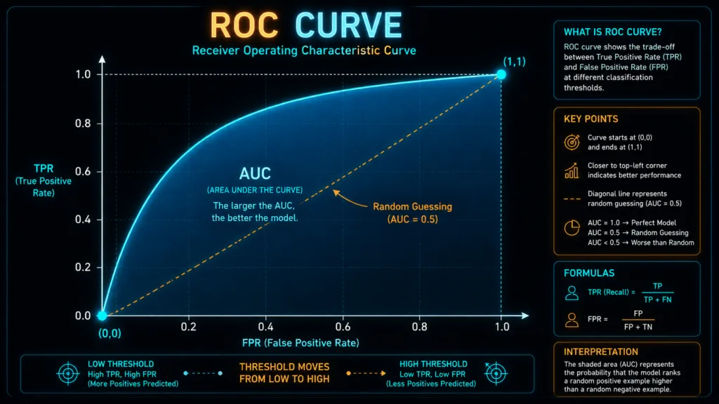
The Key Insight: Every threshold you choose (say, 0.5) gives you a confusion matrix. Each confusion matrix gives you a point (FPR, TPR). The ROC curve is just all these points connected.
But the area under this curve? That’s where things get spicy.
3. The Curve: TPR vs FPR
Before the math, let’s define our monsters:
True Positive Rate (TPR) = Recall = Sensitivity = TP / (TP + FN)
“Of all actual positives, what fraction did my model catch?”
False Positive Rate (FPR) = FP / (FP + TN)
“Of all actual negatives, what fraction did my model falsely flag as positive?”
The ROC curve plots TPR on the y-axis and FPR on the x-axis, sweeping over every possible threshold.
4. The Mind-Bending Claim
Here’s what we’re about to prove:
AUC = P(score_positive > score_negative)
Where score_positive is the score assigned to a randomly chosen positive example, and score_negative is the score assigned to a randomly chosen negative example.
In other words: If you pick one positive and one negative at random, the AUC is the probability that your model gives a higher score to the positive one.
The name for this: This is exactly the probability that your model correctly ranks a random positive-negative pair.
5. The Geometric Proof
Let’s build intuition before we touch algebra.
Step 1: Fix a Threshold
Choose any threshold t. At this threshold:
The TPR tells you what fraction of positives score ≥ t
The FPR tells you what fraction of negatives score ≥ t
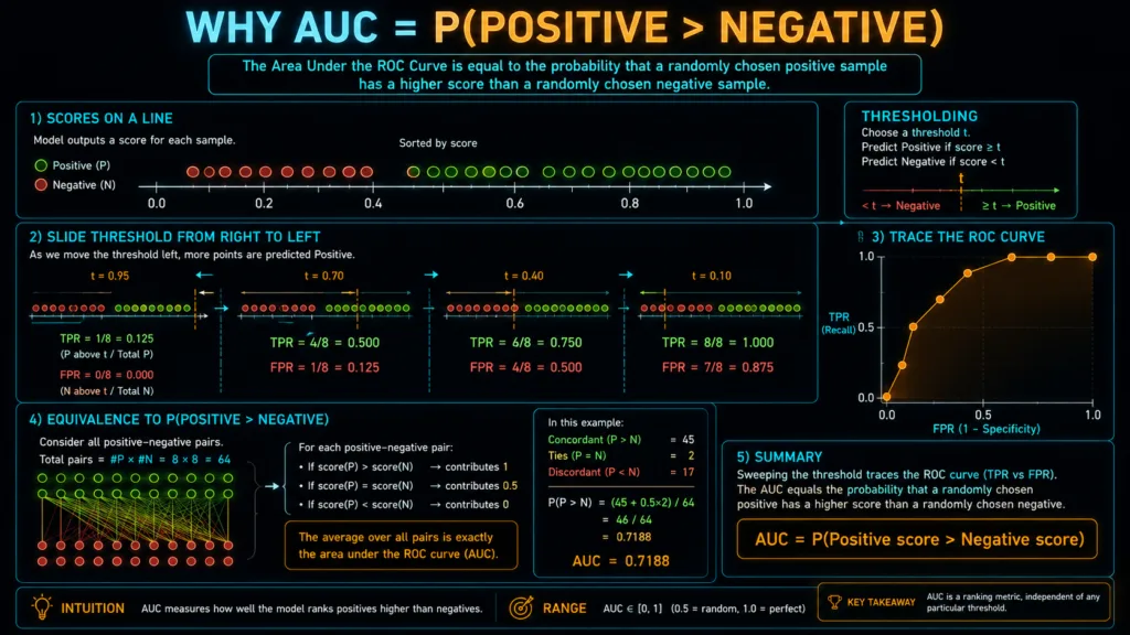
Visualize this: Imagine all positive scores as green dots on a number line, and all negative scores as red dots. Threshold t is a vertical cut.
Step 2: The Two-Part Construction
Instead of integrating over thresholds (which is what the area under the curve does), imagine randomly picking a positive and a negative.
If you pick a positive with score s_p and a negative with score s_n, you want to know: is s_p > s_n?
Step 3: The Probability as an Integral
For a fixed positive score s_p, the probability that a randomly chosen negative has a score less than s_p is:
P(s_n < s_p | s_p) = FPR at threshold s_p
Why? Because FPR(s_p) is exactly the fraction of negatives with score ≥ s_p, so 1 - FPR(s_p) is the fraction with score < s_p.
Wait. That’s not quite right. Let me fix that.
Step 4: The Correct Geometric Interpretation
For a fixed threshold t, TPR(t) is the fraction of positives with score ≥ t, and FPR(t) is the fraction of negatives with score ≥ t.
The integral form of AUC is:
The key insight: dFPR(t) represents the density of negative scores at threshold t.
Step 5: The “Area = Probability” Realization
When you perform the integration over all thresholds, you are effectively:
Picking a random negative example (contributing the
dFPR)For that negative with score
s_n, adding up the fraction of positives whose score is >s_n(which isTPR(s_n))
This is exactly the probability that a random positive beats a random negative!
🤧 Allergic to algebra? I’ve got you. If you’re a visual learner who needs to see it to believe it, jump into our [MATHS & GRAPHS FOR ML – neuralninjas.in – neuralninjas.in Lab for ML at Neural Ninjas]. Zero math headaches, 100% visual intuition!
6. The Algebraic Proof (The Math)
Now let’s get our hands dirty.
Step 1: Define the Sets
Let there be P positive examples and N negative examples.
Let f be the scoring function from our model.
Step 2: Express AUC as a Sum Over Pairs
The area under the ROC curve can be expressed as:
Where I is the indicator function (1 if true, 0 otherwise).
This is exactly the definition of P(positive_score > negative_score)!
Step 3: What This Means
The number of correctly ordered positive-negative pairs divided by the total number of positive-negative pairs IS the probability.
This is why scikit-learn can compute AUC without drawing a graph. It just sorts all predictions, counts how many positive-negative pairs are ordered correctly, and divides by the total.
Step 4: The Ranking Formulation
If we have a sorted list of predictions, the computation becomes:
AUC = (sum of ranks of positive examples) - (P × (P + 1) / 2) / (P × N)
This is exactly the Mann-Whitney U statistic normalized.
7. The Mann-Whitney U Connection:
The U Statistic
The Mann-Whitney U statistic counts the number of times a positive example outscores a negative example:
The Normalization
This is the direct bridge: The geometric area under the ROC curve equals the normalized Mann-Whitney U statistic.
Why This Matters
The U statistic is a standard non-parametric test for comparing two distributions
AUC inherits all the properties of the U test
AUC is distribution-free – it doesn’t assume any shape for the data
8. What About Ties? The 0.5 Rule
The Problem: Your model predicts exactly 0.75 for both a positive and a negative example. How do we count this pair?
The Rule: Award it 0.5. The pair is neither correctly ranked nor incorrectly ranked. It’s a tie.
Mathematical Implementation
def calculate_auc(scores, labels):
    # Sort by score descending
    sorted_indices = sorted(range(len(scores)), key=lambda i: scores[i], reverse=True)

    pos_count = sum(labels)
    neg_count = len(labels) - pos_count

    # Handle ties by averaging ranks
    ranks = [0] * len(labels)
    i = 0
    while i < len(sorted_indices):
        j = i
        # Find all tied scores
        while j < len(sorted_indices) and scores[sorted_indices[j]] == scores[sorted_indices[i]]:
            j += 1
        # Assign average rank
        avg_rank = (i + j + 1) / 2  # 1-indexed ranks
        for k in range(i, j):
            ranks[sorted_indices[k]] = avg_rank
        i = j

    # Sum ranks for positive examples
    pos_rank_sum = sum(ranks[i] for i in range(len(labels)) if labels[i] == 1)

    # AUC = (sum_pos_ranks - pos_count * (pos_count + 1) / 2) / (pos_count * neg_count)
    auc = (pos_rank_sum - pos_count * (pos_count + 1) / 2) / (pos_count * neg_count)

    return auc
The 0.5 Rule in Action: Ties get averaged ranks, which effectively counts them as 0.5 in the U statistic.
9. The Imbalance Paradox: When AUC Lies to You
The Setup:
Your dataset has 99% negatives and 1% positives. Your model predicts everything as negative. What happens?
Accuracy: 99% (Looks amazing!)
AUC: 0.5 (Totally random)
Why AUC Stays at 0.5
AUC is invariant to class imbalance. Let’s prove it.
Proof Sketch:
In the ranking formulation:
P positives and N negatives
AUC = U / (P × N)
If all scores are equal, every positive-negative pair is a tie:
Each tie contributes 0.5 to U
U = P × N × 0.5
AUC = 0.5
Class imbalance doesn’t matter. AUC is calculated over PAIRS, not individual examples. Each pair contributes equally, so the class ratio doesn’t affect the probability.
The Flip Side: When AUC Misleads You
If you have a very imbalanced dataset and care about finding rare positives, AUC can look deceptively perfect.
Example:
P = 100, N = 10,000
Model ranks only 50% of positives above negatives
AUC = 0.5 (Random!)
But if all 100 positives are in the top 1000 predictions, the Precision-Recall curve will tell a very different story.
10. AUC vs PR-AUC: The High-Stakes Battle
The Difference
| Metric | What It Measures | When It Matters |
|---|---|---|
| ROC-AUC | Ranking performance (positive vs negative pairs) | General performance, balanced data |
| PR-AUC | Precision-Recall tradeoff | Imbalanced data, rare positives |
The Math Behind the Difference:
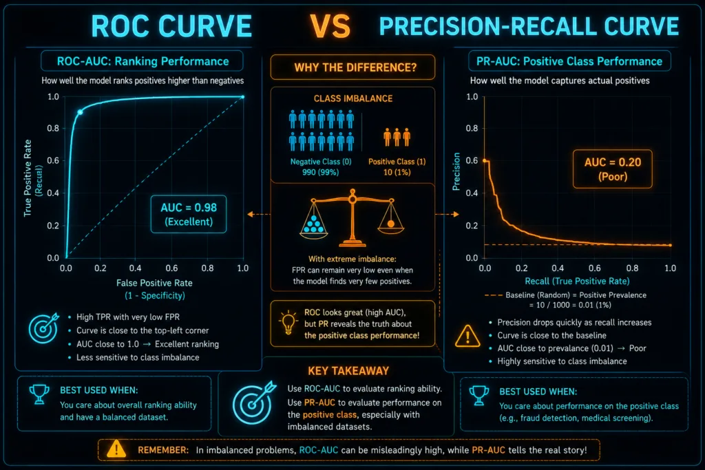
ROC-AUC weighs TPR and FPR equally. A huge number of true negatives makes FPR small, inflating the score.
PR-AUC uses Precision (TP/(TP+FP)) and Recall (TP/(TP+FN)). It ignores true negatives entirely.
Why ROC-AUC Can Be High While PR-AUC Is Low
ROC-AUC = 0.98
PR-AUC = 0.20
This happens when:
Many true negatives (imbalanced data)
Model only catches a fraction of positives
But false positive rate is still low due to many negatives
The Insight: ROC-AUC tells you about ranking. PR-AUC tells you about practical performance on the positive class.
11. Code: Computing AUC Without Drawing a Graph
scikit-learn Implementation:
from sklearn.metrics import roc_auc_score
import numpy as np

# Example predictions and labels
predictions = np.array([0.1, 0.4, 0.35, 0.8, 0.2, 0.6])
labels = np.array([0, 0, 1, 1, 0, 1])

# Standard function
auc = roc_auc_score(labels, predictions)
print(f"ROC-AUC: {auc:.4f}")

# Here's what's happening under the hood:
def manual_auc(y_true, y_score):
    # Get positive and negative scores
    pos_scores = y_score[y_true == 1]
    neg_scores = y_score[y_true == 0]

    # Count correctly ordered pairs
    correct = 0
    ties = 0
    for pos in pos_scores:
        for neg in neg_scores:
            if pos > neg:
                correct += 1
            elif pos == neg:
                ties += 1

    # AUC = (correct + 0.5 * ties) / (len(pos_scores) * len(neg_scores))
    return (correct + 0.5 * ties) / (len(pos_scores) * len(neg_scores))

manual = manual_auc(labels, predictions)
print(f"Manual AUC: {manual:.4f}")  # Should match roc_auc_score
The Efficient Ranking Algorithm
def fast_auc(y_true, y_score):
    """
    Compute AUC efficiently using sorting.
    Handles ties with average ranks (0.5 rule).
    """
    # Get indices sorted by score descending
    order = np.argsort(y_score)[::-1]
    sorted_labels = y_true[order]

    # Compute ranks with tie handling
    ranks = np.zeros(len(y_score))
    i = 0
    while i < len(order):
        j = i
        # Find all tied scores
        while j < len(order) and y_score[order[j]] == y_score[order[i]]:
            j += 1
        # Assign average rank
        avg_rank = (i + j + 1) / 2  # 1-indexed ranks
        for k in range(i, j):
            ranks[order[k]] = avg_rank
        i = j

    # Sum ranks for positives
    pos_ranks = ranks[y_true == 1]
    pos_count = len(pos_ranks)
    neg_count = len(y_true) - pos_count

    # AUC = (sum_pos_ranks - pos_count * (pos_count + 1) / 2) / (pos_count * neg_count)
    return (pos_ranks.sum() - pos_count * (pos_count + 1) / 2) / (pos_count * neg_count)

# Test it
print(f"Fast AUC: {fast_auc(labels, predictions):.4f}")
Visualizing the ROC Curve
import matplotlib.pyplot as plt
from sklearn.metrics import roc_curve

def plot_roc_curve(y_true, y_score, title="ROC Curve"):
    fpr, tpr, thresholds = roc_curve(y_true, y_score)
    auc = roc_auc_score(y_true, y_score)

    plt.figure(figsize=(8, 6))
    plt.plot(fpr, tpr, label=f"ROC Curve (AUC = {auc:.3f})", linewidth=2)
    plt.plot([0, 1], [0, 1], 'k--', label="Random Guessing", linewidth=1)
    plt.xlabel("False Positive Rate (FPR)")
    plt.ylabel("True Positive Rate (TPR)")
    plt.title(title)
    plt.legend()
    plt.grid(alpha=0.3)
    plt.show()

plot_roc_curve(labels, predictions)
12. The Edge Cases: AUC = 0.5, AUC = 0.0, AUC = 1.0
AUC = 1.0: Perfect Separability
Every positive example has a higher score than every negative example. Perfect ranking.
Mathematically: U = P × N, so AUC = 1.0
AUC = 0.5: Random Guessing
The model’s scores are completely independent of the labels. The number of correctly ranked pairs equals the number of incorrectly ranked pairs.
Mathematically: U = P × N / 2, so AUC = 0.5
AUC = 0.0: Perfectly Inverted
Every positive has a LOWER score than every negative. The model is perfectly wrong.
Mathematically: U = 0, so AUC = 0.0
The Fix: If your AUC is 0.0, just flip the predictions! (1 – predictions). You’ll get AUC = 1.0.
The Brainteaser :
“What does an AUC of 0.0 mean mathematically?”
If AUC = P(positive > negative) = 0.0, then it’s never true that a positive outscores a negative. This means every negative outscores every positive. The model is perfectly inverted.
In practice, an AUC of 0.0 is just as impressive as an AUC of 1.0 – it means the model has learned something perfect but opposite.
13. The Interview Question (And How to Crush It)
The Setup
The interviewer writes on the whiteboard:
“Prove that ROC-AUC equals P(positive_score > negative_score).”
Your Step-by-Step Answer
Step 1 – The Geometry (30 seconds)
“The area under the ROC curve is defined as the integral of TPR with respect to FPR. When we integrate over all thresholds, we’re effectively summing over all possible negative examples.”
Step 2 – The Probability Interpretation (30 seconds)
“For a fixed negative example with score s, TPR(s) is exactly the fraction of positives with score > s. So by integrating over all negatives (which is what dFPR does), we’re counting, for each negative, how many positives beat it.”
Step 3 – The Algebra (1 minute)
“Let P be the number of positives and N the number of negatives. The AUC can be written as:
AUC = (1/(P×N)) × Σ_{pos} Σ_{neg} I(score_pos > score_neg)This is exactly the definition of the probability that a random positive outscores a random negative.”
Step 4 – The Mann-Whitney Connection (30 seconds)
“This is also the normalized Mann-Whitney U statistic. The U statistic counts exactly the number of positive-negative pairs where the positive outscores the negative. Normalizing by P×N gives us the AUC.”
Step 5 – The Tie Handling (30 seconds)
“If there are ties, we award 0.5 to each tied pair, which is why scikit-learn’s roc_auc_score has a ‘drop’ parameter for handling ties.”
The Bonus: What This Tells Us
“AUC is distribution-free. It doesn’t depend on class imbalance. It’s a measure of ranking quality, not classification quality. That’s why it’s great for comparing models but can be misleading for imbalanced data.”
14. FAQs: The Questions Everyone Asks
Why does ROC-AUC equal P(positive > negative)?
Because the area under the ROC curve is exactly the integral that counts how many positive-negative pairs are correctly ranked. The integration over all thresholds sums over all possible comparisons.
What’s the Mann-Whitney U connection?
AUC = U / (P × N), where U is the Mann-Whitney statistic counting how many positives outscores negatives. This is why AUC can be computed without plotting a curve.
What happens when there are ties in predictions?
Ties are awarded 0.5. A tied positive-negative pair is counted as half-correct, half-incorrect. This is implemented by assigning average ranks to ties.
Why does class imbalance not affect AUC?
AUC is computed over pairs (positive, negative), not over individual examples. Each pair contributes equally regardless of class counts. This makes AUC invariant to class imbalance.
Why can ROC-AUC be high while PR-AUC is low?
ROC-AUC looks at TPR vs FPR. A huge number of true negatives makes FPR small even if you miss many positives. PR-AUC looks at Precision and Recall, which are affected by the number of positives found. In imbalanced data, PR-AUC is more informative.
How does scikit-learn compute AUC without drawing a graph?
It uses the ranking algorithm: sort predictions, compute ranks, sum ranks for positives, and use the Mann-Whitney formula. No graph is actually drawn.
What does AUC = 0.5 mean?
Your model is no better than random guessing. It ranks positives and negatives equally well (or equally poorly).
What does AUC = 0.0 mean?
Your model is perfectly inverted. Every negative outscores every positive. Flip your predictions and you get AUC = 1.0.
Can two different models have the same AUC but different performance?
Yes. AUC is an average over all thresholds. Two models can have the same AUC but perform very differently at specific operating points. One might be excellent at low FPR while the other is mediocre everywhere.
Why do I have to be careful with AUC for imbalanced data?
Because AUC ignores class imbalance, it can look perfect while you’re missing all the rare positives. If you care about finding rare positives, use PR-AUC instead.
15. The Bottom Line:
The TL;DR
The geometric area under the ROC curve EQUALS the probability that a random positive ranks higher than a random negative.
| Concept | What It Is | Why It Matters |
|---|---|---|
| ROC Curve | TPR vs FPR for all thresholds | Visualizing ranking performance |
| AUC | Area under the ROC curve | Summary metric for ranking |
| P(positive > negative) | Probability of correct ranking | What AUC actually measures |
| Mann-Whitney U | Count of correctly ranked pairs | How AUC is computed |
| Class Imbalance | AUC ignores it | Why AUC can mislead |
ROC-AUC is the probability that a randomly chosen positive ranks higher than a randomly chosen negative.
This is mathematically proven by showing the area integral equals the pair-count formula.
Use PR-AUC instead when your data is imbalanced and you care about finding rare positives.
The Final Word
The area under the ROC curve isn’t just a geometric area. It’s a probability. It’s the Mann-Whitney U statistic. It’s the chance that your model correctly orders a random positive-negative pair.
And when you understand that, you understand why AUC is such a powerful and widely-used metric. It’s not just about curves. It’s about ranking.