PyTorch Activation Functions: The Neuron’s Personality and Why They Matter

Demystify PyTorch activation functions! Learn why they’re crucial for non-linearity, which ones to use, and how to avoid common pitfalls like vanishing gradients and dying ReLUs.

      Table of Contents

• Introduction: What’s Missing from Your Neural Network?
• Activation Functions in the Real World
• The Core Concept: Why Your Network Needs Non-Linearity
• The Cast of Characters: A Guide to Common Activation Functions
• The Villains: Common Problems & How to Fight Them
• Choosing Your Weapon: A Practical Flowchart
• Hyperparameters to Tweak
• Putting It All Together in PyTorch
• Summary & Key Takeaways

Introduction: What’s Missing from Your Neural Network?

Ever feel like your neural network is just… nodding along, agreeing with everything, but never really understanding? You’ve stacked layers, added neurons, and tweaked weights, but it’s still giving you bland, linear answers. What’s missing? It’s the spark, the personality, the decision-maker in your network: the activation function! Think of it like the “on/off” switch or the “dimmer” for your neurons. Without these crucial functions, your deep learning model is just a fancy calculator, incapable of learning anything truly complex. Ready to inject some personality and learning power into your PyTorch models and finally understand why these seemingly simple functions are the secret sauce to deep learning magic?

Activation Functions in the Real World

Before we dive into the code and math, let’s see where these “neuron personalities” are already at work. They aren’t just academic concepts; they power the apps and technology you use daily.

• BookMyShow’s Demand Forecasting: When a new movie trailer drops, how does BookMyShow predict ticket demand in Mumbai versus Bengaluru? Their models analyze hype, historical data, and showtimes. Activation functions like ReLU help these models capture complex, non-linear relationships, like how demand doesn’t just increase steadily but can spike suddenly based on factors like trailer popularity or star power. ReLU’s ability to pass positive signals through directly, while zeroing out negative inputs, helps the system decide if the “hype signal” is strong enough to “activate” a prediction for a sold-out show.
• PhonePe & Paytm’s Anomaly Detection: How do these UPI apps flag a potentially fraudulent transaction? A simple linear model can’t catch sophisticated scams. Neural networks use activation functions like Sigmoid to squash neuron outputs into a specific, bounded range. This is crucial for anomaly detection where multiple factors (unusual transaction time, strange location, large amount) are weighed. Sigmoid helps the model synthesize these disparate signals into a nuanced “risk score” to decide if the combined “risk signal” is high enough to trigger an alert.
• Tesla’s Autopilot Vision System: When a Tesla identifies a pedestrian, a stop sign, or another car, it’s using a deep convolutional neural network. Activation functions, especially variants of ReLU (like Leaky ReLU), are critical here. They allow the network to learn intricate visual features—the sharp edge of a curb, the specific hue of a traffic light—by deciding which visual information is important enough to pass to the next layer. If a neuron detects a strong edge, ReLU passes that signal forward; if the signal is weak, it’s suppressed, allowing the network to focus on the most salient visual cues.

The Core Concept: Why Your Network Needs Non-Linearity

So, what exactly is an activation function? In the simplest terms, an activation function is a mathematical function applied to the output of a neuron. It decides whether the neuron should be “activated” or not, and what signal it should pass to the next layer.

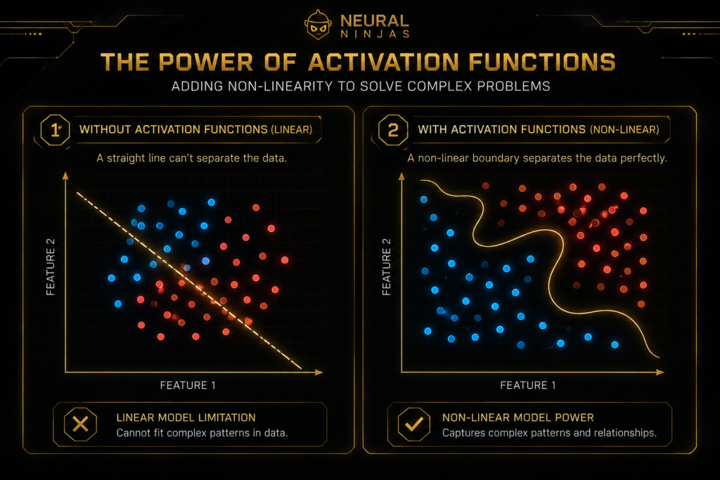
Think of it like this: Imagine you’re sorting mail. A simple rule might be “If the letter is heavy, put it in the ‘packages’ pile.” That’s a linear decision. But what if the rule is “If the letter is heavy AND it’s a small box, OR if it’s a light envelope with a ‘fragile’ sticker, put it in the ‘special handling’ pile”? That’s a complex, non-linear decision. A neural network without activation functions can only make simple, “heavy vs. light” decisions. No matter how many layers you add, you’re just stacking simple rules on top of each other, which still results in one simple rule. Activation functions give your network the ability to learn those complex “AND/OR” rules, allowing it to understand the messy, non-linear patterns of the real world.

The Cast of Characters: A Guide to Common Activation Functions

Let’s meet the most common activation functions you’ll encounter in PyTorch. For every function, we’ll break down exactly what it is, why it’s important, and how it actually works, so you can make smart decisions for your own models.

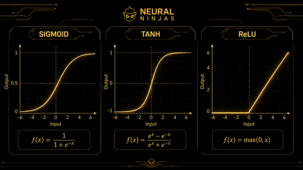
1. Sigmoid (The Classic Squeezer) :-The Sigmoid function is one of the oldest and most fundamental activation functions. Think of it as a “probability converter.”

• WHAT is it? Sigmoid is a mathematical function that takes any real number as input and “squashes” it into a range between 0 and 1. It produces a smooth “S”-shaped curve.
• f(x)=11+e−x f(x) = \frac{1}{1 + e^{-x}} f(x)=1+e−x1​
• WHY does it matter? Its primary purpose is to convert a raw numerical output (called a logit) into a probability. An output of 0.7 from a Sigmoid function can be interpreted as a 70% probability that a given input belongs to the positive class.
• HOW does it work?

  1. If the input x is a large positive number, e^(-x) becomes tiny, and the output is close to 1.

  2. If x is a large negative number, e^(-x) becomes huge, and the output is close to 0.

  3. If x is exactly 0, the output is 0.5.

• WHEN to use it?

  * Use it: Almost exclusively in the output layer of a binary classification model (e.g., “spam” vs. “not spam”).

  * Do NOT use it: In the hidden layers of deep neural networks. It leads to the “vanishing gradient” problem.

• ADVANTAGES

  * Probabilistic Interpretation: Its output range of [0, 1] is perfect for representing a probability.

  * Smooth Gradient: It’s differentiable everywhere, which is required for training.

• LIMITATIONS

  * Vanishing Gradients: The slope of the curve is nearly flat for very high or low inputs. In deep networks, these tiny gradients get multiplied and “vanish,” preventing early layers from learning.

  * Not Zero-Centered: The output is always positive, which can slow down the learning process.

2. Tanh (The Centered Squeezer):- Tanh, or the hyperbolic tangent function, is like Sigmoid’s cousin but with a key difference in its output range.

• WHAT is it? Tanh squashes any real number into a range between -1 and 1. It’s also an “S”-shaped curve, but it’s centered around zero. f(x)=ex−e−xex+e−x f(x) = \frac{e^x – e^{-x}}{e^x + e^{-x}} f(x)=ex+e−xex−e−x​
• WHY does it matter? It was an improvement over Sigmoid. Because its output is centered around zero, it often helps the learning process converge faster. A neuron’s output can be strongly negative, neutral, or strongly positive, giving the next layer a more balanced signal.
• HOW does it work?

  1. If the input x is a large positive number, the output gets very close to 1.

  2. If the input x is a large negative number, the output gets very close to -1.

  3. If the input x is 0, the output is exactly 0.

• WHEN to use it?

  * Use it: Historically popular in the hidden layers of shallow networks, especially Recurrent Neural Networks (RNNs).

  * Do NOT use it: In modern, very deep networks. It still suffers from the vanishing gradient problem. ReLU and its variants have almost completely replaced it.

• ADVANTAGES

  * Zero-Centered Output: Its [-1, 1] range helps center the data for the next layer, which typically makes learning faster than with Sigmoid.

  * Steeper Gradient: The slope is steeper than Sigmoid’s around zero, leading to stronger initial gradients.

• LIMITATIONS

  * Vanishing Gradients: Just like Sigmoid, the function flattens out for large inputs, causing the gradient to vanish in deep networks.

3. ReLU (The Modern Default):- ReLU, or the Rectified Linear Unit, is the undisputed champion of modern deep learning. Its simplicity is its greatest strength.

• WHAT is it? ReLU is a very simple function. If the input is positive, it returns the input. If the input is negative or zero, it returns zero. $f(x)=\max (0,x)$
• WHY does it matter? ReLU was a breakthrough because it solved the vanishing gradient problem for positive inputs. Since the function doesn’t “saturate” (flatten out) for positive values, the gradient doesn’t shrink to zero. This allows for training much deeper networks.
• HOW does it work? It’s like a simple switch:

  1. If a neuron’s input x is positive (e.g., 5.2), it passes 5.2 to the next layer. The “switch” is on.

  2. If x is negative (e.g., -3.1), it passes 0 to the next layer. The “switch” is off.

• WHEN to use it?

  * Use it: This should be your default choice for all hidden layers in almost any neural network. Always start with ReLU.

  * When NOT to use it: Be cautious if many neurons are outputting zero during training (the “Dying ReLU” problem).

• ADVANTAGES

  * Computationally Efficient: It’s just a max(0, x) operation, which is extremely fast.

  * No Vanishing Gradient (for positive inputs): For any positive input, the gradient is a constant 1, allowing the learning signal to propagate.

  * Sparsity: By outputting 0 for negative inputs, it can make the network more efficient.

• LIMITATIONS

  * The Dying ReLU Problem: If a neuron’s weights are updated so its input is always negative, it will always output 0. Its gradient will also be 0, so it stops learning entirely. It effectively “dies.”

  * Not Zero-Centered: Its outputs are always non-negative.

4. Leaky ReLU (The Fix for a Dying Network):- Leaky ReLU is a simple but effective modification of ReLU designed to address its biggest weakness.

• WHAT is it? A variant of ReLU that, instead of outputting 0 for negative inputs, outputs a very small positive value (the input multiplied by a small constant, $\alpha$). $f(x)=\max (\alpha x,x)$ Here, $\alpha$ is a small constant (like 0.01).
• WHY does it matter? It was created specifically to solve the “Dying ReLU” problem. By allowing a small, non-zero gradient to flow through the neuron even when its input is negative, it ensures that the neuron can never truly “die.”
• HOW does it work?

  1. If the input x is positive (e.g., 5.2), it behaves like ReLU and outputs 5.2.

  2. If x is negative (e.g., -3.1), instead of outputting 0, it outputs $\alpha \times x\text{[}\alpha \times x$. For $\alpha =0.01$\alpha=0.01 ], the output would be $-0.031\text{[}-0.031$. This is the “leak.”

• WHEN to use it?

  * Use it: As a direct replacement for ReLU, especially if your model is not training well or you suspect neurons are dying. It’s a slightly safer choice.

  * When NOT to use it: There are very few downsides. In practice, it’s almost always a good alternative to try.

• ADVANTAGES

  * Prevents Dying Neurons: Its primary benefit is keeping neurons alive and learning.

  * Maintains Benefits of ReLU: It is still computationally fast and avoids the vanishing gradient problem.

• LIMITATIONS

  * Extra Hyperparameter: The $\alpha$\alpha ] value is another parameter you might need to tune, though the default usually works well.

  * Inconsistent Performance: Its superiority over ReLU is not always guaranteed and can be task-dependent.

5. Softmax (The Multi-Class Decider):- Softmax is different. It doesn’t operate on a single number; it operates on a whole vector of numbers at the very end of the network.

• WHAT is it? Softmax takes a vector of raw scores (logits) and converts them into a probability distribution, where each element is between 0 and 1, and all elements sum to 1. σ(z)i=ezi∑j=1Kezj \sigma(\mathbf{z})i = \frac{e^{z_i}}{\sum{j=1}^{K} e^{z_j}} σ(z)i=∑j=1Kezj​ezi​​
• WHY does it matter? It’s the standard way to get a probabilistic output for a multi-class classification problem. If you’re classifying an image as a “cat,” “dog,” or “bird,” Softmax will give you the probability for each class (e.g., [0.1, 0.8, 0.1], meaning an 80% chance it’s a dog).
• HOW does it work?

  1. It takes the raw outputs from the last layer (e.g., [2.0, 1.0, 0.1]).

  2. It calculates the exponential of each number: [7.39, 2.72, 1.11]. This highlights the largest score.

  3. It sums these values: 11.22.

  4. It divides each exponential value by the sum to normalize them into probabilities: [0.66, 0.24, 0.10].

• WHEN to use it?

  * Use it: Exclusively in the output layer of a multi-class classification model, where an input can only belong to one of several classes.

  * Do NOT use it: In hidden layers or for binary classification (use Sigmoid).

• ADVANTAGES

  * Probabilistic Output: Provides a clear, interpretable probability distribution over all classes.

  * Highlights Largest Logit: The exponentiation step leads to a more confident prediction.

• LIMITATIONS

  * Output Layer Only: It is not a general-purpose activation for hidden layers.

  * Assumes Mutually Exclusive Classes: It forces probabilities to sum to 1, so it’s only for problems where classes are mutually exclusive (an image is a cat OR a dog, not both).

The Villains:

Common Problems & How to Fight Them Even with the right activation function, things can go wrong. Here are the two biggest “villains” you’ll face and how to defeat them.

1. The Vanishing / Exploding Gradient Problem This is the classic villain that plagued early deep learning and is the main reason Sigmoid and Tanh fell out of favor for deep networks.

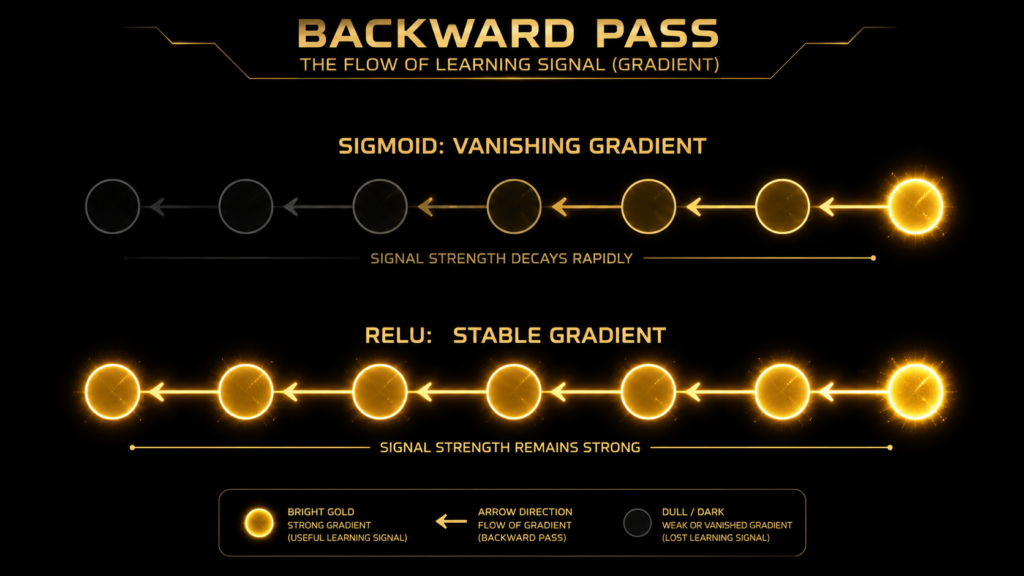
• WHAT is it? The Vanishing Gradient problem occurs when the signals used to update the network’s weights become extremely small as they are passed backward during training. The Exploding Gradient problem is the opposite: the gradients become excessively large.
• WHY does it matter? If the gradient vanishes, the weights of the first few layers don’t get updated. This means the layers responsible for learning the most basic features (like edges and colors in an image) are essentially frozen. Your deep network behaves like a shallow one.
• HOW does it work? Training involves multiplying gradients at each layer. The derivative of the Sigmoid function is always ≤ 0.25. In a deep network, you multiply many numbers less than 0.25 together (e.g., 0.2 * 0.15 * 0.22 * …), and the product shrinks exponentially to almost zero.
• HOW do you fix it? — Use ReLU or its variants: This is the #1 solution. The derivative of ReLU is 1 for positive inputs, so the gradient doesn’t shrink.  Proper Weight Initialization: Techniques like “He” or “Xavier” initialization help prevent gradients from starting off too small or large.
• Batch Normalization: This technique normalizes the output of a layer, keeping gradients in a healthy range.

2. The Dying ReLU Problem This villain is a specific side effect of using the otherwise heroic ReLU function.

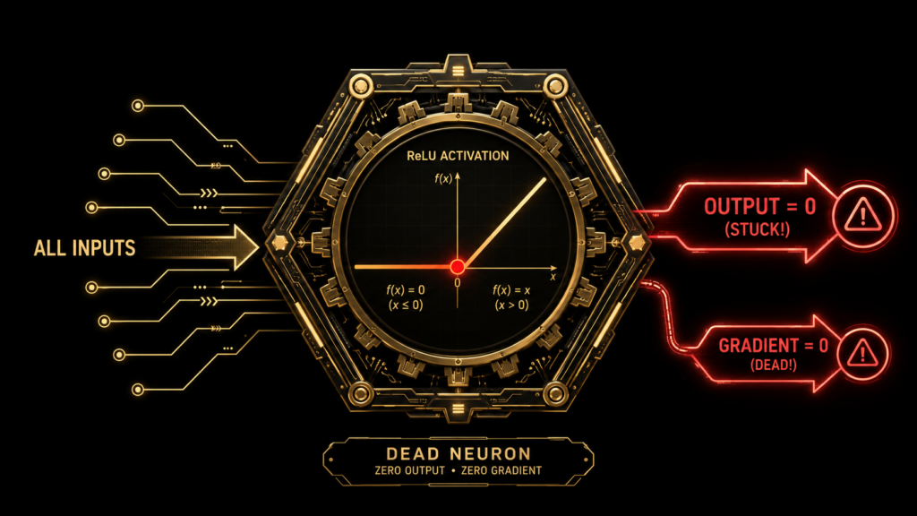
• WHAT is it? A “dead” ReLU neuron is one that gets stuck always outputting 0 for every data point. Once this happens, the gradient flowing through it will also be 0 forever, and it can never update its weights again.
• WHY does it matter? A dead neuron is a useless neuron. It stops learning permanently. If a significant portion of your neurons die, you are effectively reducing the size and capacity of your network, which can severely hurt performance.
• HOW does it work? A large gradient update (often from a high learning rate) might change a neuron’s weights so drastically that its input becomes negative for all training examples. Once the input is always negative, the ReLU function always outputs 0, and the gradient is always 0. The neuron is permanently stuck.
• HOW do you fix it?

  * Use Leaky ReLU (or its variants): This is the most direct solution. It ensures there is always a small, non-zero gradient for negative inputs, allowing the neuron to recover.

* Lower the Learning Rate: Smaller learning rates lead to more gentle weight updates, making it less likely that a neuron gets pushed into a “dead” state.

  * Use Adaptive Learning Rate Optimizers: Optimizers like Adam automatically adjust the learning rate, which can help prevent the large, destructive updates that cause neurons to die.

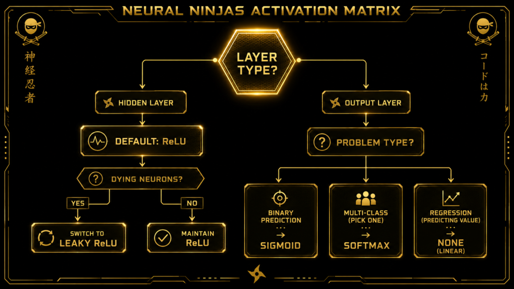
Choosing Your Weapon:

A Practical Flowchart Feeling overwhelmed? Use this simple flowchart to guide your decisions.

Hyperparameters to Tweak

While most activation functions are parameter-free, some have dials to turn. The most common is:

• alpha in Leaky ReLU: This is the “leak” coefficient—the small slope for negative inputs. In PyTorch (nn.LeakyReLU), this is the negative_slope parameter, which defaults to 0.01. You can experiment with slightly larger or smaller values to see if it helps your model avoid dying neurons more effectively.

Imagine a pipe that shuts off if pressure is too low (standard ReLU). Leaky ReLU adds a tiny emergency drain to that pipe. The alpha value is the size of that drain. It keeps a little bit of flow going, preventing a total blockage. Putting It All Together in PyTorch Let’s see how simple it is to use these functions in a real PyTorch model.

import torch
import torch.nn as nn

# A simple neural network for demonstration
class SimpleClassifier(nn.Module):
    def __init__(self):
        super(SimpleClassifier, self).__init__()
        # Layer 1: 10 input features, 32 output features
        self.layer1 = nn.Linear(in_features=10, out_features=32)
        # Activation 1: Our go-to for hidden layers!
        self.activation1 = nn.ReLU() 
        
        # Layer 2: 32 input features, 16 output features
        self.layer2 = nn.Linear(in_features=32, out_features=16)
        # Activation 2: An alternative to try if ReLUs are dying
        self.activation2 = nn.LeakyReLU(negative_slope=0.01) 
        
        # Output Layer: 16 input features, 2 output features (for 2 classes)
        self.output_layer = nn.Linear(in_features=16, out_features=2)
        
        # Note: We don't apply Softmax here because the loss function
        # nn.CrossEntropyLoss() does it for us efficiently.
        # If this were a binary classifier, the output_features would be 1
        # and we would apply nn.Sigmoid() after the final layer.

    def forward(self, x):
        x = self.layer1(x)
        x = self.activation1(x)
        x = self.layer2(x)
        x = self.activation2(x)
        x = self.output_layer(x)
        return x

# Let's create an instance of our model
model = SimpleClassifier()
print(model)

# --- How to use different activations for an output layer ---

# For Binary Classification (e.g., Spam vs. Not Spam)
# output_layer = nn.Linear(in_features=16, out_features=1)
# output_activation = nn.Sigmoid()

# For Multi-Class Classification (e.g., Cat vs. Dog vs. Bird)
# output_layer = nn.Linear(in_features=16, out_features=3)
# output_activation = nn.Softmax(dim=1) # Applied to the output tensor

This code shows how activation functions are just another layer in your nn.Module stack. PyTorch handles all the complex backpropagation math for you, so you can focus on designing the right architecture.

The Activation Function Race :-

Here are three key learnings that we can grasp by watching this visualization:

1. Gradient Saturation (The “Vanishing” Problem): By observing the Sigmoid and Tanh points, we will see that as the input (x) moves far away from zero, the points barely move vertically even though the input continues to increase. This visualizes gradient saturation, where the output becomes flat, effectively killing the learning signal for deep layers.

2. The “Fast Lane” Efficiency: we can notice how ReLU (and Leaky ReLU) continue to climb steeply as inputs become positive. This visually demonstrates why ReLU is the “Fast Lane”—it doesn’t have a squashing limit (asymptotic bound) like Sigmoid or Tanh, which allows gradients to flow through the network much more efficiently without being throttled.

3. Survival of the Negative Signal: By watching the Leaky ReLU point in the negative region ($x < 0$), we can see it doesn’t stay stuck at zero like the standard ReLU. This provides an immediate visual explanation for why we use Leaky ReLU: it keeps a “trickle” of information alive even for negative inputs, preventing the “Dying ReLU” problem where neurons get stuck and stop learning forever.

Summary & Key Takeaways

• Activation Functions are Essential: They introduce non-linearity, allowing your network to learn complex patterns. Without them, your network is just a simple linear model.
• ReLU is Your Default: For hidden layers, always start with nn.ReLU(). It’s fast and avoids the vanishing gradient problem.
• Watch Out for Dying ReLUs: If your model struggles to train, some neurons might be “dead.” Switch to nn.LeakyReLU() to fix this.
• Choose the Right Output Function: Use nn.Sigmoid() for binary classification and nn.Softmax() for multi-class classification. For regression (predicting a continuous number), use no activation function on the output layer.
• Avoid Sigmoid/Tanh in Deep Hidden Layers: They are prone to the vanishing gradient problem and have been largely replaced by ReLU and its variants.

By understanding the personality and purpose of each activation function, you’re no longer just copy-pasting code; you’re making informed architectural decisions that will dramatically improve your PyTorch models. Keywords: PyTorch activation functions, ReLU, Sigmoid, Tanh, Leaky ReLU, Softmax, non-linearity, neural networks, deep learning, vanishing gradients, dying ReLU problem, PyTorch tutorial.