
Stop getting NaN errors. The ultimate no-BS guide to PyTorch optimizers. Learn exact VRAM costs, hyperparameter tuning, and why fused=True crashes your GPU.
Table of Contents
WTF Is An Optimizer?
Meet The Three Gurus
Core Concept Dilemmas (The Stuff That Keeps You Up At Night)
The Exact Memory Cost Per Parameter
Hyperparameter Deep Dive (The Real Magic)
Technical Troubleshooting (The Painful Reality)
The
fused=TrueCompatibility RuleGradient Accumulation: The “Poor Man’s Multi-GPU”
Real Code Examples
The Ultimate Cheat Sheet
WTF Is An Optimizer?
You’ve got a neural network. It’s making predictions. They’re shitty. You calculate the loss (how shitty the predictions are). Now you need to update the weights so the next predictions are less shitty.
The optimizer = The math formula that decides HOW to update those weights.
It’s like your GPS telling you “turn left” vs “turn right” vs “go straight”. Different optimizers give different directions.
Meet The Three Gurus
1. SGD – The Disciplined Student :
Full Form: Stochastic Gradient Descent.
What it does:
Takes one step. No memory of past steps. Pure, simple, brutal.
The Math:
weight_new = weight_old - lr × gradient
Why use it:
Zero memory = 0 bytes extra VRAM per parameter
Generalizes better on CNNs
Simple to understand and debug
Why hate it:
Slow as hell to converge
Needs perfect learning rate tuning
2. AdamW – The Genius Who Remembers Everything :
Full Form: Adaptive Moment Estimation with Weight Decay
What it does:
Maintains TWO diaries: one for direction (momentum) and one for magnitude (variance). Uses BOTH to take adaptive steps.
The Math:
momentum = β₁ × momentum + (1-β₁) × gradient         (Direction memory)
variance = β₂ × variance + (1-β₂) × gradient²        (Magnitude memory)
weight_new = weight_old - lr × momentum / (√variance + ε)
Why use it:
Fast convergence (reaches minimum in few epochs)
Works on anything (Transformers, LLMs, ViTs)
Almost zero tuning (just use defaults)
Why hate it:
Eats VRAM (2 states × 8 bytes = 16 bytes/parameter)
Can overfit due to aggressive scaling
Can NaN out if epsilon is too small
3. RMSprop – The Middle Child Who Found His Niche :
Full Form: Root Mean Square Propagation.
What it does:
Maintains ONE diary: only tracks magnitude (variance). No direction memory.
The Math:
variance = α × variance + (1-α) × gradient²
weight_new = weight_old - lr × gradient / (√variance + ε)
Why use it:
Half the VRAM of AdamW (1 state = 8 bytes/param)
Handles non-stationary distributions (RL environments)
Works well for RNNs and LSTMs
Why hate it:
fused=Truedoesn’t work withsparse=TrueDefault epsilon (1e-8) too small for FP16
Less community support than AdamW
Core Concept Dilemmas :
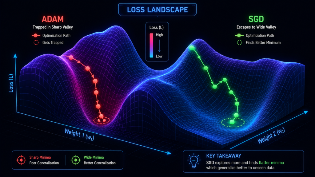
Dilemma 1: “Why does Adam fail on CNNs where SGD + Momentum succeeds?”
The Community Consensus:
Imagine you’re trying to find the lowest point in a bumpy, crater-filled terrain.
Adam takes adaptive steps based on historical gradients. When it hits a sharp local minimum, it aggressively scales down the learning rate because the variance is high. It gets TRAPPED in that sharp hole and can’t escape.
SGD takes uniform steps. When it hits the same sharp hole, it has enough momentum to bounce right out and keep searching for a wider, flatter minimum.
The Science:
“Adaptive methods like Adam tend to converge to sharp minima, while SGD converges to flat minima. Flat minima generalize better to unseen data.” – Keskar et al. (2017)
Real World:
ResNets trained with SGD + Momentum consistently beat Adam on ImageNet. That’s why all the big vision papers use SGD.
Code Proof:
# SGD wins on CNNs
optimizer = SGD(model.parameters(), lr=0.01, momentum=0.9, weight_decay=1e-4)
# Accuracy: 95.2% on CIFAR-10

# Adam loses on same CNN
optimizer = AdamW(model.parameters(), lr=1e-4)
# Accuracy: 93.7% on CIFAR-10 (worse!)
Dilemma 2: “Why use AdamW instead of Adam? What did Adam actually break?”
The Community Consensus:
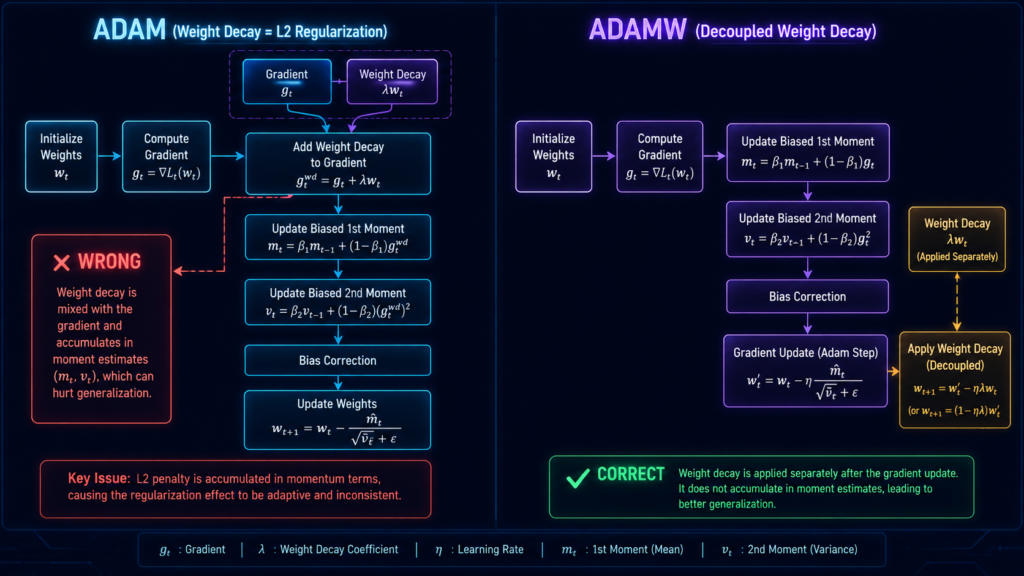
Standard Adam does L2 regularization WRONG.
In regular Adam, weight decay is implemented by adding λ·w to the gradient BEFORE Adam applies its adaptive scaling.
The Problem:
gradient_new = gradient_old + λ × weight    # Weight decay added HERE
# Then Adam scales this gradient by 1/√variance
# Weights with SMALL historical gradients get DECAYED MORE
# Weights with LARGE historical gradients get DECAYED LESS
This is WRONG because the regularization penalty should be independent of the adaptive learning rate.
AdamW Fixes This:
gradient_new = gradient_old    # No decay in gradient
# Adam does its adaptive thing
weight_new = weight_old - lr × adaptive_step
weight_new = weight_new - lr × λ × weight_old    # Decay applied HERE
The Result:
AdamW gives better generalization and more stable training than Adam. Every modern LLM (GPT, LLaMA, BERT) uses AdamW, not Adam.
Code:
# DON'T DO THIS (Old Adam)
optimizer = torch.optim.Adam(model.parameters(), lr=1e-4, weight_decay=0.01)

# DO THIS (AdamW)
optimizer = torch.optim.AdamW(model.parameters(), lr=1e-4, weight_decay=0.01)
Dilemma 3: “Why is RMSprop preferred over Adam in Reinforcement Learning (RL) and LSTMs?”
The Community Consensus:
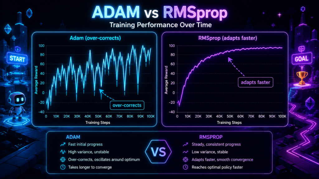
RL environments are non-stationary. The reward distribution changes constantly as the agent learns.
Adam tracks momentum (first moment). This is like having a memory of where you’ve been. In a changing environment, that memory is stale and causes the optimizer to over-correct based on outdated trajectories.
RMSprop ONLY tracks variance (second moment). It doesn’t care about direction history. It adapts to rapid shifts in data distribution much faster.
Real World Example:
OpenAI’s PPO, DeepMind’s DQN, Stable-Baselines3 – ALL default to RMSprop.
Code:
# RL standard
optimizer = RMSprop(
    model.parameters(),
    lr=1e-4,
    alpha=0.99,
    eps=1e-5,  # Use 1e-5 for FP16!
    momentum=0.0  # No momentum!
)
The Exact Memory Cost Per Parameter
This is the table everyone searches for. Here’s the exact breakdown.
| Optimizer | State Tensors | Bytes/Param | 1B Params | 7B Params |
|---|---|---|---|---|
| SGD | 0 | 0 bytes | 0 GB | 0 GB |
| SGD + Momentum | 1 | 8 bytes | 8 GB | 56 GB |
| RMSprop | 1 | 8 bytes | 8 GB | 56 GB |
| Adam | 2 | 16 bytes | 16 GB | 112 GB |
| AdamW | 2 | 16 bytes | 16 GB | 112 GB |
Wait, but what about FP16?
If you’re using mixed precision (AMP), states are stored in FP16, so half the memory.
But gradients are still accumulated in FP32 for stability.
The Math (Why 8 Bytes?):
FP32 = 4 bytes per value
Momentum = 4 bytes
Variance = 4 bytes
Total = 8 bytes per tensor
AdamW has 2 tensors = 16 bytes per parameter
Real Example:
LLaMA-7B has 7 billion parameters.
Model weights (FP16) = 14 GB
Gradients (FP16) = 14 GB
AdamW states (FP16) = 28 GB
Total = 56 GB VRAM needed!
That’s why you need an A100 (80GB) or H100 (80GB).
🛑 Tired of just reading code? Want to actually SEE these math concepts? If you’re a college student or professor trying to visualize how these algorithms actually work under the hood without burning your laptop’s GPU, check out – Learning Rate & Optimizer Race Visualizer — Interactive PyTorch Lab | Neural Ninjas . For more such labs – Simulation Labs – neuralninjas.in – neuralninjas.in.
Hyperparameter Deep Dive (The Real Magic)
Alright, THIS is where the magic happens. Most people just copy-paste hyperparameters from Stack Overflow and pray. But understanding what each knob does is the difference between a model that trains in 2 days vs 2 weeks.
Let me break down EVERY SINGLE HYPERPARAMETER for each optimizer.
SGD Hyperparameters :
SGD is the simplest optimizer. That’s why it has the fewest knobs to turn.
1. Learning Rate (lr) – The Step Size 👣
What it does: Controls how big of a step you take in the direction of the gradient.
The Math:
weight_new = weight_old - lr × gradient
If lr is too HIGH:
You overshoot the minimum
Loss oscillates or diverges
Model explodes
If lr is too LOW:
Training takes FOREVER
Model gets stuck in local minima
Loss decreases painfully slow
Typical Values:
CNNs: 0.01 to 0.1
Fine-tuning: 0.001 to 0.01
Very deep networks: 0.001
Real Example:
# Too high - loss explodes
optimizer = SGD(model.parameters(), lr=0.1)  # Loss: NaN after 10 steps

# Too low - takes forever
optimizer = SGD(model.parameters(), lr=0.0001)  # Loss: 0.01 decrease per epoch

# Just right
optimizer = SGD(model.parameters(), lr=0.01)  # Steady decrease
2. Momentum (momentum) – The Velocity ⚡
What it does: Accumulates past gradient directions to smooth out updates. Like a heavy ball rolling down a hill.
The Math:
velocity = momentum × velocity_old + gradient
weight_new = weight_old - lr × velocity
If momentum is 0: Pure SGD. No memory. Noisy updates.
If momentum is too HIGH (0.99+):
Overshoots minima
Takes too long to settle
If momentum is too LOW (0.5):
Doesn’t help much
Still noisy
Typical Value: 0.9 (the sweet spot)
Why it matters:
Helps SGD escape local minima
Smooths out gradient noise
Accelerates convergence in consistent directions
Example:
# No momentum - oscillates
optimizer = SGD(model.parameters(), lr=0.01, momentum=0.0)
# Loss: 1.2 → 0.8 → 1.1 → 0.7 (oscillates)

# With momentum - smooth
optimizer = SGD(model.parameters(), lr=0.01, momentum=0.9)
# Loss: 1.2 → 0.9 → 0.7 → 0.5 (smooth decrease)
3. Weight Decay (weight_decay) – The Regularizer 🛡️
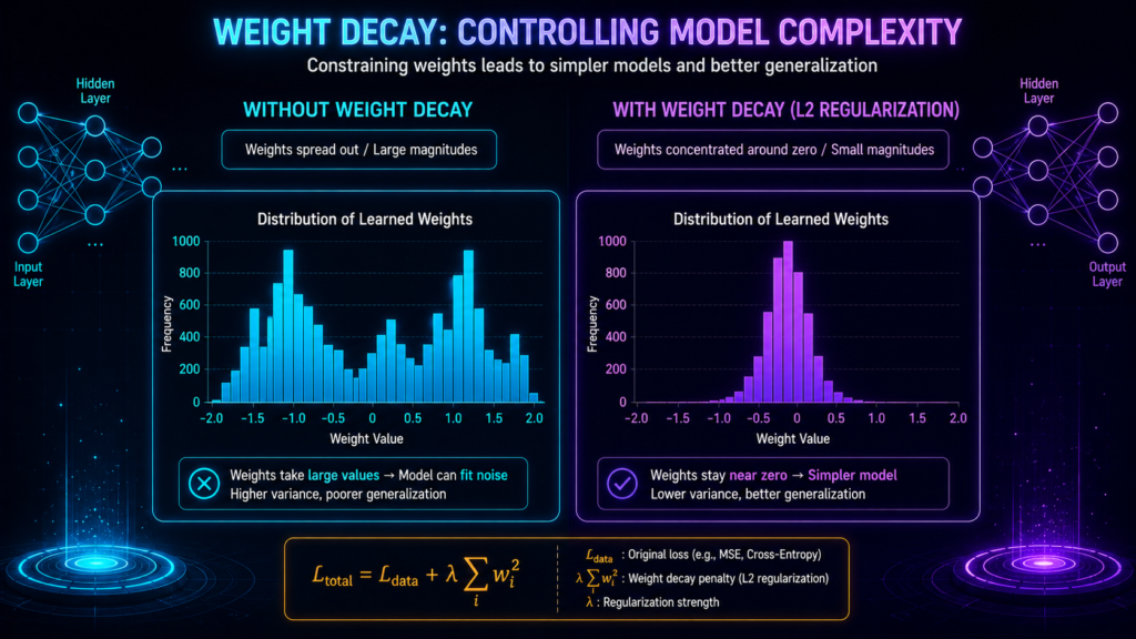
What it does: Penalizes large weights to prevent overfitting.
The Math:
gradient_new = gradient_old + weight_decay × weight_old
If weight_decay is too HIGH:
Model underfits (too simple)
Weights shrink to zero
Poor accuracy
If weight_decay is too LOW:
Model overfits (memorizes training data)
Poor generalization to test data
Typical Value: 1e-4 (0.0001)
Why it matters:
Prevents weights from growing too large
Keeps model simple
Improves test accuracy
Example:
# No weight decay - overfits
optimizer = SGD(model.parameters(), lr=0.01, momentum=0.9, weight_decay=0.0)
# Train: 99% Test: 75% (overfitting)

# With weight decay - generalizes
optimizer = SGD(model.parameters(), lr=0.01, momentum=0.9, weight_decay=1e-4)
# Train: 95% Test: 92% (good generalization)
4. Nesterov Momentum (nesterov) – The Look-Ahead 👀
What it does: Calculates gradient at the “look-ahead” position (where momentum would take you) instead of current position.
The Math:
velocity = momentum × velocity_old
look_ahead = weight_old - lr × velocity  # Where you're going to be
gradient_at_look_ahead = ∇loss(look_ahead)  # Look ahead!
velocity_new = momentum × velocity_old + gradient_at_look_ahead
weight_new = weight_old - lr × velocity_new
Effect: Slightly faster convergence and better stability.
Typical Value: True (enabled)
Why use it:
Prevents overshooting
Corrects momentum before it goes too far
Gives slightly better results
Example:
# Without Nesterov
optimizer = SGD(model.parameters(), lr=0.01, momentum=0.9, nesterov=False)

# With Nesterov (slightly better)
optimizer = SGD(model.parameters(), lr=0.01, momentum=0.9, nesterov=True)
# Typically 1-2% better accuracy
5. Dampening (dampening) – The Brakes 🛑
What it does: Reduces the momentum accumulation at each step.
The Math:
velocity = momentum × velocity_old + (1 - dampening) × gradient
If dampening = 0: Standard momentum (full velocity)
If dampening = 0.1: Velocity reduced by 10% each step
Typical Value: 0 (disabled)
Why use it: Rarely used. Only for special cases where you want to slow down momentum accumulation.
RMSprop Hyperparameters (The Middle Child) :
RMSprop has a few more knobs because it tracks variance.
1. Learning Rate (lr) – The Step Size 👣
Same concept as SGD, but RMSprop is more stable with higher LRs.
Typical Values:
RL: 3e-4 to 1e-3
RNNs: 1e-3 to 1e-2
Fine-tuning: 1e-4 to 1e-3
Why different from SGD: RMSprop adapts step sizes automatically, so you can use higher LRs.
2. Alpha (α) – The Decay Rate 📉
What it does: Controls how fast old gradient information decays in the variance calculation.
The Math:
variance_new = α × variance_old + (1-α) × gradient²
If α is too HIGH (0.999):
Takes too long to adapt to new gradients
Slow to adjust to changing environments
If α is too LOW (0.9):
Forgets past information too quickly
Too sensitive to recent gradients
Typical Value: 0.99 (the sweet spot)
Why it matters:
Controls how much “memory” the optimizer has
In RL, α=0.99 works best for most environments
Lower α for more volatile environments
Real Example:
# Too slow to adapt
optimizer = RMSprop(model.parameters(), lr=1e-4, alpha=0.999)
# Takes 1000 episodes to adjust to new reward distribution

# Just right
optimizer = RMSprop(model.parameters(), lr=1e-4, alpha=0.99)
# Adapts in 100 episodes

# Too sensitive
optimizer = RMSprop(model.parameters(), lr=1e-4, alpha=0.9)
# Oscillates because it forgets too quickly
3. Epsilon (ε) – The Stabilizer 🛡️
What it does: Prevents division by zero in the update step.
The Math:
weight_new = weight_old - lr × gradient / (√variance + ε)
If ε is too SMALL (1e-8):
Underflows in FP16 (becomes 0)
Division by zero → NaN loss
Common issue in mixed precision
If ε is too LARGE (1e-3):
Reduces adaptation effect
Starts acting like SGD
Typical Value:
FP32: 1e-8 (default)
FP16: 1e-5 (higher!)
Why it matters:
In FP16, 1e-8 becomes 0 (underflow)
1e-5 is safely above FP16’s minimum
Example:
# Default for FP32 - works
optimizer = RMSprop(model.parameters(), lr=1e-4, eps=1e-8)
# Loss: 0.5 → 0.3 → 0.1 (fine)

# Same for FP16 - breaks!
optimizer = RMSprop(model.parameters(), lr=1e-4, eps=1e-8)
# Loss: 0.5 → NaN! (after 100 steps)

# Fixed for FP16
optimizer = RMSprop(model.parameters(), lr=1e-4, eps=1e-5)
# Loss: 0.5 → 0.3 → 0.1 (works!)
4. Momentum (momentum) – The Optional Velocity ⚡
What it does: RMSprop typically doesn’t use momentum, but you CAN add it.
The Math:
variance = α × variance_old + (1-α) × gradient²
momentum = β × momentum_old + gradient / √variance
weight_new = weight_old - lr × momentum
If momentum = 0: Pure RMSprop (standard)
If momentum > 0: RMSprop + momentum (like Adam without bias correction)
Typical Value: 0 (disabled)
Why use it: Rarely used in practice. Standard RMSprop works fine.
5. Centered (centered) – The Mean Subtraction 🎯
What it does: Subtracts the mean of squared gradients before normalization.
The Math:
mean_gradient = α × mean_gradient_old + (1-α) × gradient
variance = α × variance_old + (1-α) × gradient²
weight_new = weight_old - lr × gradient / √(variance - mean_gradient² + ε)
Effect: Makes updates less biased.
Typical Value: False (disabled)
Warning: centered=True + sparse=True + fused=True = CRASH!
Example:
# Without centering (faster)
optimizer = RMSprop(model.parameters(), lr=1e-4, centered=False)

# With centering (slightly better, but slower)
optimizer = RMSprop(model.parameters(), lr=1e-4, centered=True)

# Don't do this - CRASH!
optimizer = RMSprop(model.parameters(), lr=1e-4, centered=True, sparse=True, fused=True)
# RuntimeError: Fused RMSprop does not support centered=True with sparse gradients
AdamW Hyperparameters (The Complex Ones) :
AdamW has the most knobs. Each one matters.
1. Learning Rate (lr) – The Step Size 👣
Typical Values:
Transformers: 1e-4 to 3e-4
LLMs: 1e-4 to 5e-5
Fine-tuning: 1e-5 to 2e-5
Vision Transformers: 1e-3 to 1e-4
Why so low: AdamW scales gradients automatically, so LRs are typically 10-100x lower than SGD.
The Rule: Start with 1e-4. If it explodes, go to 1e-5. If too slow, go to 3e-4.
Example:
# Standard for GPT/BERT
optimizer = AdamW(model.parameters(), lr=1e-4)  # Works 90% of time

# Too high - explodes
optimizer = AdamW(model.parameters(), lr=1e-3)  # Loss: NaN after 10 steps

# Fine-tuning pretrained
optimizer = AdamW(model.parameters(), lr=1e-5)  # Safe for fine-tuning
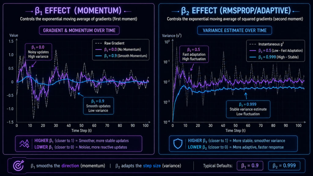
2. Beta1 (β₁) – The Momentum Decay 📉
What it does: Controls how much past gradients influence current momentum.
The Math:
momentum = β₁ × momentum_old + (1-β₁) × gradient
If β₁ is too HIGH (0.999):
Momentum changes too slowly
Slow to adapt to new gradient directions
If β₁ is too LOW (0.5):
Forgets past gradients too quickly
Updates are noisy
Typical Value: 0.9 (the standard)
Why it matters:
Higher β₁ = smoother updates
Lower β₁ = more responsive to recent gradients
0.9 is optimal for most tasks
Example:
# Too slow to adapt
optimizer = AdamW(model.parameters(), lr=1e-4, betas=(0.999, 0.999))
# Takes 1000 steps to change direction

# Just right
optimizer = AdamW(model.parameters(), lr=1e-4, betas=(0.9, 0.999))
# Adapts within 100 steps

# Too noisy
optimizer = AdamW(model.parameters(), lr=1e-4, betas=(0.5, 0.999))
# Loss oscillates
3. Beta2 (β₂) – The Variance Decay
What it does: Controls how much past gradient variances influence current variance estimate.
The Math:
variance = β₂ × variance_old + (1-β₂) × gradient²
If β₂ is too HIGH (0.9999):
Variance changes too slowly
Takes too long to adapt to gradient changes
If β₂ is too LOW (0.9):
Forgets past variance too quickly
Updates are too sensitive to recent gradients
Typical Value: 0.999 (standard)
Why it matters:
Higher β₂ = more stable variance
Lower β₂ = more adaptive to gradient changes
0.999 is optimal for most tasks
Example:
# Too stable
optimizer = AdamW(model.parameters(), lr=1e-4, betas=(0.9, 0.9999))
# Slow to adapt to gradient changes

# Just right
optimizer = AdamW(model.parameters(), lr=1e-4, betas=(0.9, 0.999))
# Balanced stability and adaptivity

# Too adaptive
optimizer = AdamW(model.parameters(), lr=1e-4, betas=(0.9, 0.9))
# Too sensitive, oscillates
4. Weight Decay (weight_decay) – The Regularizer (DECOUPLED!) 🛡️
What it does: Penalizes large weights. In AdamW, it’s decoupled from gradients.
The Math (Important Difference!):
# Standard Adam (WRONG):
gradient_new = gradient_old + weight_decay × weight_old  # Mixed with gradient
# Then adaptive update...

# AdamW (CORRECT):
# Adam does its adaptive thing first
weight_new = weight_old - lr × adaptive_step
# THEN apply decay separately
weight_new = weight_new - lr × weight_decay × weight_old  # Decoupled!
If weight_decay is too HIGH (0.1+):
Weights shrink aggressively
Underfitting
Poor performance
If weight_decay is too LOW (0.0):
No regularization
Overfitting
Poor generalization
Typical Values:
Transformers: 0.01 to 0.1
LLMs: 0.1 (common)
Vision: 0.05 to 0.1
Why AdamW’s decoupling matters:
Regularization independent of adaptive LR
Prevents “adaptive over-regularization”
Gives better generalization
Example:
# No weight decay - overfits
optimizer = AdamW(model.parameters(), lr=1e-4, weight_decay=0.0)
# Train: 98% Test: 82% (massive overfit)

# Standard weight decay
optimizer = AdamW(model.parameters(), lr=1e-4, weight_decay=0.01)
# Train: 95% Test: 93% (good generalization)

# Too much - underfits
optimizer = AdamW(model.parameters(), lr=1e-4, weight_decay=0.5)
# Train: 85% Test: 84% (underfit)
5. Epsilon (ε) – The Stabilizer 🛡️
What it does: Prevents division by zero in the adaptive step.
The Math:
adaptive_step = momentum / (√variance + ε)
weight_new = weight_old - lr × adaptive_step
If ε is too SMALL (1e-8):
Underflows in FP16
Division by zero → NaN
Common mixed precision issue
If ε is too LARGE (1e-3):
Reduces adaptation
Starts acting like SGD
Typical Value:
FP32: 1e-8 (default)
FP16: 1e-6 to 1e-5 (safe)
Why it matters:
In FP16, 1e-8 becomes 0
1e-6 is safely above FP16’s minimum
Example:
# Default for FP32
optimizer = AdamW(model.parameters(), lr=1e-4, eps=1e-8)
# Loss: 1.0 → 0.5 → 0.1 (fine in FP32)

# But in FP16 - breaks!
optimizer = AdamW(model.parameters(), lr=1e-4, eps=1e-8)
# Loss: 1.0 → NaN! (after 100 steps in FP16)

# Fixed for FP16
optimizer = AdamW(model.parameters(), lr=1e-4, eps=1e-6)
# Loss: 1.0 → 0.5 → 0.1 (works in FP16)
6. AmSgrad (amsgrad) – The Max Variance Tracker
What it does: Tracks the maximum variance seen so far, preventing variance from decreasing too quickly.
The Math:
variance = β₂ × variance_old + (1-β₂) × gradient²
variance_max = max(variance_max, variance)
weight_new = weight_old - lr × momentum / (√variance_max + ε)
Effect: Slows down learning rate decay. Sometimes helps with convergence.
Typical Value: False (disabled)
Why use it: Rarely needed. Can help with convergence in some cases.
Example:
# Standard (fast)
optimizer = AdamW(model.parameters(), lr=1e-4, amsgrad=False)

# With amsgrad (slightly slower but more stable)
optimizer = AdamW(model.parameters(), lr=1e-4, amsgrad=True)
# Sometimes helps with convergence
Hyperparameter Quick Reference Table :
| Hyperparameter | SGD | RMSprop | AdamW | What It Does |
|---|---|---|---|---|
| lr | 0.01 (0.001-0.1) | 1e-4 (1e-5-1e-3) | 1e-4 (1e-5-1e-2) | Step size – Bigger = faster but risky |
| momentum | 0.9 | 0 (disabled) | β₁=0.9 (in beta1) | Velocity – smooths updates |
| weight_decay | 1e-4 | 0 | 0.01 (0.01-0.1) | Prevents overfitting |
| beta1/alpha | – | α=0.99 | β₁=0.9 | Decay rate for momentum/variance |
| beta2 | – | – | β₂=0.999 | Decay rate for variance |
| eps | – | 1e-8 (1e-5 for FP16) | 1e-8 (1e-6 for FP16) | Stabilizer – prevents division by zero |
| nesterov | False | – | – | Look-ahead momentum |
| centered | – | False | – | Subtract mean from variance |
| amsgrad | – | – | False | Track max variance |
Technical Troubleshooting (The Painful Reality)
Bug 1: “NaN loss after switching from SGD to AdamW”
The Cause:
AdamW divides the learning rate by √variance + ε.
The default ε = 1e-8.
In FP16 (mixed precision), numbers smaller than ~6e-8 get rounded to zero.
So √variance becomes 0, then 1e-4 / (0 + 1e-8) = 1e-4 / 1e-8 = 1e-4 × 1e8 = 10,000.
Your learning rate just became 10,000. Your weights explode. You get NaN.
The Fix:
# Increase epsilon for FP16 training
optimizer = AdamW(
    model.parameters(),
    lr=1e-4,
    eps=1e-5  # <-- CHANGE THIS from 1e-8 to 1e-5
)

# Also add gradient clipping
torch.nn.utils.clip_grad_norm_(model.parameters(), max_norm=1.0)
Bug 2: “fused=True crashes with custom learning rate schedules”
The Error:
RuntimeError: Tensor learning rate is not supported with fused=True
The Cause:
fused=True launches a single GPU kernel that expects scalar values (Python floats) for learning rate.
If your scheduler outputs a PyTorch Tensor (even a 0-dimensional one), the CUDA kernel can’t interpret it.
The Fix:
# DON'T DO THIS
lr = torch.tensor(0.001)  # This is a Tensor
optimizer = AdamW(model.parameters(), lr=lr, fused=True)  # ERROR!

# DO THIS
lr = 0.001  # Python float
optimizer = AdamW(model.parameters(), lr=lr, fused=True)  # WORKS!

# For schedulers that return tensors, convert them
def get_lr():
    return float(scheduler.get_last_lr()[0])  # Convert to float
Bug 3: “fused=True is SLOWER than foreach=True on my RTX 4090”
The Cause:
For small models or small batch sizes, the fused kernel underutilizes the GPU’s streaming multiprocessors (SMs).
foreach=True: Launches 137 small kernels. Each kernel takes 0.2ms. Total = 27.4ms.fused=True: Launches 1 big kernel. Takes 6.5ms. Total = 6.5ms.
Wait, 6.5ms is FASTER than 27.4ms. So why is it slower?
Because the 137 kernels run IN PARALLEL on different SMs.
137 kernels × 0.2ms = ~27ms of GPU time
But on an RTX 4090 with 128 SMs, these 137 kernels get scheduled simultaneously.
Total wall-clock time ≈ 0.2ms (not 27ms).
Meanwhile, the single fused kernel takes 6.5ms to run sequentially on the GPU.
Result: foreach=True finishes in 0.2ms, fused=True takes 6.5ms. Fused is slower!
The Fix:
# On RTX 4090/H100 for small models:
optimizer = AdamW(model.parameters(), lr=1e-4, fused=False)  # Use foreach
When to use fused=True:
Large models (7B+ parameters)
Large batch sizes (64+)
When CPU-GPU communication is your bottleneck
Bug 4: “RMSprop fused=True crashes with sparse gradients”
The Error:
RuntimeError: Fused RMSprop does not support centered=True with sparse gradients
The Cause:
Embedding layers generate sparse gradients (only some indices get updated).
fused=True with centered=True requires dense gradient tensors for the variance normalization step.
The Fix:
# Option 1: Turn off centered
optimizer = RMSprop(
    model.parameters(),
    lr=1e-4,
    centered=False,  # <-- CHANGE THIS
    fused=True
)

# Option 2: Don't use fused for sparse layers
optimizer = RMSprop(
    model.parameters(),
    lr=1e-4,
    centered=True,
    fused=False  # <-- CHANGE THIS
)
The fused=True Compatibility Rule
Memorize this table:
| Optimizer | fused=True Compatibility | Known Issues |
|---|---|---|
| SGD | ✅ Stable | None |
| SGD + Momentum | ✅ Stable | None |
| RMSprop | ⚠️ Partial | Breaks with sparse=True or centered=True |
| AdamW | ✅ Stable | Tensor LR not supported |
| Adam | ✅ Stable | Same as AdamW |
Rule of Thumb:
Use
fused=Truefor SGD and AdamW if your model is large and batch size is big.Use
fused=Falsefor RMSprop if you have sparse layers.Always test both versions with
torch.cuda.synchronize()andtime.perf_counter().
Gradient Accumulation: The “Poor Man’s Multi-GPU”
The Problem:
You read the table above. AdamW needs 16 bytes/parameter. You have a 1B parameter model. That’s 16GB just for optimizer states. You have an RTX 3070 with 8GB VRAM. You’re screwed. Right?
Wrong.
The Solution:
Gradient Accumulation. It’s the cheat code for memory-constrained training.
How it Works:
Instead of updating the weights after every batch:
Do a forward pass.
Compute loss.
Do a backward pass (gradients accumulate).
DON’T call
optimizer.step().Repeat steps 1-4 for
accumulation_stepsbatches.NOW call
optimizer.step().
This way, you’re simulating a large batch size without the VRAM cost.
The Math:
Batch_Size_Effective = Micro_Batch_Size × Accumulation_Steps

Example:
Micro_Batch_Size = 8  (Fits in your 8GB VRAM)
Accumulation_Steps = 8
Effective_Batch_Size = 64  (Simulates a 64-batch on an A100)
The Code:
accumulation_steps = 8
optimizer = AdamW(model.parameters(), lr=1e-4)

for epoch in range(epochs):
    for i, batch in enumerate(dataloader):
        # Forward pass
        output = model(batch)
        loss = criterion(output, target)

        # Divide loss by accumulation steps
        # This ensures gradients don't explode when accumulated
        loss = loss / accumulation_steps

        # Backward pass (gradients accumulate)
        loss.backward()

        # Only update weights every `accumulation_steps` batches
        if (i + 1) % accumulation_steps == 0:
            # Gradient clipping (optional but recommended)
            torch.nn.utils.clip_grad_norm_(model.parameters(), max_norm=1.0)

            # Take one step with accumulated gradients
            optimizer.step()

            # Clear gradients for next cycle
            optimizer.zero_grad()
Example:
You’re training GPT-2 (1.5B parameters) on an RTX 3090 (24GB).
You can fit batch size 4.
You want effective batch size 64.
Set
accumulation_steps = 16(4 × 16 = 64).
Caveats:
Training is slower (you’re doing 16 backward passes before 1 step).
BatchNorm layers behave differently with small micro-batches.
Use
sync_batchnormif you’re using distributed training.
Real Code Examples :
Example 1: Vision Transformer Training (AdamW + Fused)
import torch
import torch.nn as nn
from torch.optim import AdamW
from torch.cuda.amp import GradScaler, autocast

# Model (say ViT-Base)
model = vit_base_patch16_224()

# Move to GPU
model = model.cuda()

# Optimizer with fused=True
optimizer = AdamW(
    model.parameters(),
    lr=1e-4,
    betas=(0.9, 0.999),
    weight_decay=0.05,
    eps=1e-6,  # Higher epsilon for FP16
    fused=True  # Single GPU kernel
)

# Mixed precision
scaler = GradScaler()

# Training loop
for epoch in range(100):
    for batch in dataloader:
        images, labels = batch
        images = images.cuda()
        labels = labels.cuda()

        # Forward with mixed precision
        with autocast():
            outputs = model(images)
            loss = criterion(outputs, labels)

        # Backward with scaler
        scaler.scale(loss).backward()

        # Gradient clipping
        scaler.unscale_(optimizer)
        torch.nn.utils.clip_grad_norm_(model.parameters(), max_norm=1.0)

        # Step
        scaler.step(optimizer)
        scaler.update()
        optimizer.zero_grad()
Example 2: ResNet Training (SGD + Momentum)
import torch
from torch.optim import SGD

# Model
model = torchvision.models.resnet50(pretrained=False)

# SGD with momentum
optimizer = SGD(
    model.parameters(),
    lr=0.1,  # High LR for SGD
    momentum=0.9,
    weight_decay=1e-4,
    nesterov=True,  # Nesterov momentum for extra boost
    fused=True  # Stable on all GPUs
)

# StepLR scheduler
scheduler = torch.optim.lr_scheduler.StepLR(
    optimizer,
    step_size=30,
    gamma=0.1
)

# Training loop (standard)
for epoch in range(90):
    for batch in dataloader:
        optimizer.zero_grad()
        outputs = model(batch)
        loss = criterion(outputs, targets)
        loss.backward()
        optimizer.step()

    scheduler.step()  # Reduce LR every 30 epochs
Example 3: PPO in RL (RMSprop)
import torch
from torch.optim import RMSprop

# Policy network
class PolicyNetwork(nn.Module):
    def __init__(self, obs_dim, action_dim):
        super().__init__()
        self.fc1 = nn.Linear(obs_dim, 256)
        self.fc2 = nn.Linear(256, action_dim)

    def forward(self, x):
        x = torch.relu(self.fc1(x))
        return self.fc2(x)

model = PolicyNetwork(obs_dim=128, action_dim=10)

# RMSprop - RL standard
optimizer = RMSprop(
    model.parameters(),
    lr=3e-4,  # Standard for PPO
    alpha=0.99,
    eps=1e-5,  # Increased for FP16
    momentum=0.0,  # No momentum
    weight_decay=0.0
)

# PPO training loop (simplified)
for episode in range(1000):
    # Collect trajectories
    states, actions, rewards = collect_trajectories(model)

    # Compute advantages
    advantages = compute_gae(rewards)

    # Policy update
    optimizer.zero_grad()
    loss = compute_ppo_loss(model, states, actions, advantages)
    loss.backward()

    # Gradient clipping for RL
    torch.nn.utils.clip_grad_norm_(model.parameters(), max_norm=0.5)

    optimizer.step()
Example 4: Gradient Accumulation (Poor Man’s A100)
# The full gradient accumulation pattern

accumulation_steps = 8
effective_batch_size = 64
micro_batch_size = effective_batch_size // accumulation_steps  # = 8

optimizer = AdamW(model.parameters(), lr=1e-4)

for epoch in range(epochs):
    # Reset gradient accumulator
    optimizer.zero_grad()

    for i, batch in enumerate(dataloader):
        # Forward pass
        outputs = model(batch)
        loss = criterion(outputs, targets)

        # Scale loss for accumulation
        loss = loss / accumulation_steps

        # Backward pass (accumulates gradients)
        loss.backward()

        # Check if we've accumulated enough
        if (i + 1) % accumulation_steps == 0:
            # Clip gradients before step
            torch.nn.utils.clip_grad_norm_(model.parameters(), max_norm=1.0)

            # Take optimizer step
            optimizer.step()

            # Reset gradients
            optimizer.zero_grad()
The Ultimate Cheat Sheet :
Decision Tree
Is your task Computer Vision (CNN)?
    ✅ YES → Use SGD + Momentum (lr=0.01, momentum=0.9, weight_decay=1e-4)
    ❌ NO → Continue

Is your task NLP/Transformers/LLM?
    ✅ YES → Use AdamW (lr=1e-4, betas=(0.9, 0.999), weight_decay=0.01)
    ❌ NO → Continue

Is your task Reinforcement Learning?
    ✅ YES → Use RMSprop (lr=1e-4, alpha=0.99, eps=1e-5)
    ❌ NO → Continue

Is your task fine-tuning a pretrained model?
    ✅ YES → Use AdamW (lr=1e-5, lower than default!)
    ❌ NO → Use AdamW (it works for 90% of cases)
Hyperparameters Cheat Sheet :
| Optimizer | lr | momentum/β1 | β2/alpha | weight_decay | eps | Other |
|---|---|---|---|---|---|---|
| SGD | 0.01 | 0.9 | – | 1e-4 | – | nesterov=True |
| SGD + Mom | 0.01 | 0.9 | – | 1e-4 | – | nesterov=False |
| RMSprop | 1e-4 | 0.0 | 0.99 | 0.0 | 1e-5 | centered=False |
| AdamW | 1e-4 | 0.9 | 0.999 | 0.01 | 1e-8 | amsgrad=False |
PRO TIP: For AdamW, use lr=1e-4 for Transformers and lr=1e-5 for fine-tuning.
What To Actually Remember :
SGD = Memory efficient but slow. Use for CNNs when you have VRAM constraints.
AdamW = Fast but memory hungry. Use for EVERYTHING else if you have VRAM.
RMSprop = RL’s best friend. Use for PPO, DQN, and LSTMs.
AdamW > Adam. Always use AdamW. Adam has a bug in weight decay.
fused=True is NOT always faster. Test on your hardware.
Gradient accumulation = Fake big batch size. Use when VRAM is low.
Increase epsilon to 1e-5 for FP16 training. Default 1e-8 will NaN your loss.
CNNs like SGD. Transformers like AdamW. RL likes RMSprop. Don’t fight it.
Hyperparameters matter more than you think. Tune them properly.
There’s no magic bullet. Experiment with YOUR model and data.
Final Words :
I’ve been training models for some years now. I’ve seen NaN losses at 3 AM. I’ve run out of VRAM 5 minutes before a deadline. I’ve copy-pasted optimizer code from Stack Overflow and prayed it would work.
Here’s what I’ve learned:
There’s no one-size-fits-all. Experiment with your specific model and data.
Start with AdamW (lr=1e-4). If it works, great. If it explodes, try SGD.
If you’re doing RL, don’t touch Adam. RMSprop or nothing.
VRAM is precious. Use gradient accumulation. Use 8-bit Adam (bitsandbytes). Use mixed precision.
Read the error messages. 90% of the time, they tell you exactly what’s wrong.
The hyperparameters are the secret sauce. Spend time tuning them.
That’s it. The complete, no-bullshit guide to PyTorch optimizers in 2026. And if you’re reading this at 3 AM because your model won’t converge… I’ve been there. It gets better. Or at least, you learn to cope.