
Master Learning Rate Schedulers, especially Cosine Annealing — the technique that helps your model converge smoothly to the best possible solution instead of bouncing around at the end of training.
Table of Contents
- Introduction: The Final Mile Problem
- What is a Learning Rate?
- The Core Concept: Why Static Learning Rate Fails
- Cosine Annealing — The Smart Speed Breaker
- How Cosine Annealing Works (Math Explained)
- Learning Rate Schedulers in the Real World
- Hyperparameters & Best Practices
- Common Mistakes & Gotchas
- Putting It All Together in PyTorch
- The LR Schedulers Race
- Summary & Key Takeaways
Introduction: The Final Mile Problem
You trained your model for many epochs. The loss was decreasing nicely… but suddenly in the last few epochs, it started oscillating and refused to improve further.
The culprit? Keeping the same learning rate throughout training.
Just like driving a bike at full speed on a highway and then entering your colony without slowing down — you’ll overshoot and wobble. You need to gently reduce speed near the end.
What is a Learning Rate?
When an AI makes a mistake, AutoGrad calculates the error, and the Optimizer updates the weights. The Learning Rate (LR) decides exactly how big that update step is. A big LR means massive, fast leaps. A tiny LR means slow, careful baby steps.
The Core Concept: Why Static Learning Rate Fails
A high learning rate is great in the beginning for fast exploration. But the same high learning rate near the end causes the model to overshoot the minimum, leading to oscillation and poor final performance. It will bounce back and forth across the finish line without ever actually stopping on the perfect answer.
A Learning Rate Scheduler automatically adjusts the learning rate while the AI is training. It starts fast when you have a lot of ground to cover, and automatically downshifts into a slower, more precise gear as you get closer to the perfect accuracy. Learning Rate Schedulers solve this by dynamically reducing the learning rate over time. Among them, Cosine Annealing is one of the most popular and effective.
Cosine Annealing — The Smart Speed Breaker
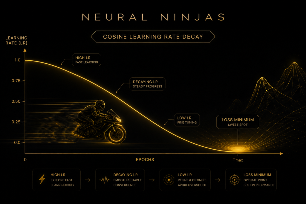
WHAT is Cosine Annealing? It decreases the learning rate following a smooth cosine curve — starting high and gently dropping to a very low value.
Analogy: When you’re riding your bike on a long highway, you go full speed. But as you approach your housing society with speed breakers and narrow turns, you don’t suddenly jam the brakes. You smoothly reduce speed in a natural curve — fast at first, then slower and more careful as you near your parking spot. That smooth deceleration is exactly what Cosine Annealing does.
How Cosine Annealing Works (Math Explained)
The formula for Cosine Annealing LR at epoch t:
ηt=ηmin+1/2(ηmax−ηmin)(1+cos(t/Tmax*π))
Where:
ηmax = Initial learning rate (the starting speed)
ηmin = Minimum learning rate (the parking speed)
Tmax = Total number of epochs
This creates a beautiful, smooth cosine wave decay — mathematically elegant and very effective in practice.
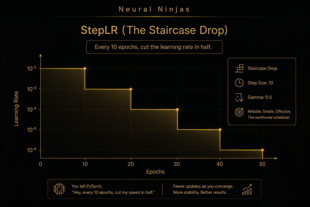
StepLR (The Staircase Drop)
This is the most famous and reliable scheduler. You tell PyTorch, “Hey, every 10 epochs, cut my speed in half.” It drops the learning rate in distinct, staircase-like steps. It is the workhorse of deep learning.
ExponentialLR (The Smooth Brake)
Instead of dropping down hard stairs, ExponentialLR applies the brakes smoothly and constantly. Every single epoch, the learning rate shrinks by a tiny fraction.
ReduceLROnPlateau (The Smart Sensor)
Most schedulers change the speed based on a timer. ReduceLROnPlateau is brilliant because it actually looks at the AI’s test scores! If the loss hasn’t improved for 5 epochs (a plateau), this scheduler yells, “We are stuck! Downshift!” and cuts the learning rate to help the AI settle into a better solution.

- When you know your training phases → StepLR
If you understand when your model should transition from exploration to fine-tuning, StepLR gives you explicit control over these phases. - When you want smooth, predictable decay → ExponentialLR
For stable, continuous reduction without sudden changes that might disrupt training momentum. - When you want to escape local minima → CosineAnnealingLR
The cosine pattern provides natural exploration phases that can help the model find better solutions. - When you’re uncertain about scheduling → ReduceLROnPlateau
This adaptive approach responds to actual training progress, making it excellent when you’re unsure about optimal timing.
For advanced optimization techniques → CyclicalLR
When you want to experiment with more sophisticated approaches that challenge traditional learning rate assumptions.
Learning Rate Schedulers in the Real World
Rapido / Ola Bike Drivers: They accelerate hard on open roads but automatically slow down near colonies, speed breakers, and tight turns. Cosine Annealing does the same for your model.
- Indian Railways: Trains run at high speed on open tracks but gradually reduce speed before reaching the station for a smooth halt.
- Tesla Autopilot: Drives fast on highways but becomes extra careful and slows down smoothly while approaching turns or parking spots.
Hyperparameters & Best Practices
- T_max: Total epochs (most important)
- eta_min: Usually a very small value like 1e-6 or 0
Pro Tip: Use CosineAnnealingWarmRestarts for long training runs — it gives the learning rate small “warm restarts” periodically.
Common Mistakes & Gotchas
Mistake: Forgetting to call scheduler.step() every epoch.
Mistake: Calling scheduler before optimizer.step() (order matters).
Putting It All Together in PyTorch
import torch
import torch.nn as nn
import torch.optim as optim
import matplotlib.pyplot as plt

# Example model
model = nn.Linear(10, 1)
optimizer = optim.Adam(model.parameters(), lr=0.01)

# Cosine Annealing Scheduler
scheduler = optim.lr_scheduler.CosineAnnealingLR(
    optimizer,
    T_max=50,      # Total number of epochs
    eta_min=1e-6   # Minimum learning rate
)

lrs = []

for epoch in range(50):
    # --- Standard Training Loop Steps ---
    # optimizer.zero_grad()
    # outputs = model(inputs)
    # loss = criterion(outputs, labels)
    # loss.backward()

    optimizer.step()          # Update weights
    scheduler.step()          # ← Update learning rate (MUST be after optimizer.step())

    current_lr = optimizer.param_groups[0]['lr']
    lrs.append(current_lr)

    if epoch % 10 == 0:
        print(f"Epoch {epoch:2d} | LR: {current_lr:.6f}")

# Plot the Learning Rate Curve
plt.figure(figsize=(10, 5))
plt.plot(lrs, color='gold', linewidth=2.5)
plt.title("Cosine Annealing Learning Rate Schedule", color='white')
plt.xlabel("Epochs")
plt.ylabel("Learning Rate")
plt.grid(True, alpha=0.3)
plt.show()
The LR Schedulers Race

🥷Summary & Key Takeaways
- Static learning rate is one of the biggest reasons models fail to converge well.
- Cosine Annealing smoothly reduces the learning rate like gently braking near a speed breaker.
- It enables fast learning in the beginning and careful fine-tuning at the end.
- Always call scheduler.step() after optimizer.step().
- Combine it with good initialization and BatchNorm for excellent results.
Keywords: Learning Rate Scheduler PyTorch, Cosine Annealing, CosineAnnealingLR, lr scheduling, deep learning optimization.