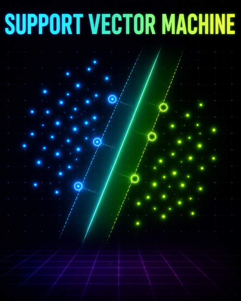
The Problem
Imagine walking through a lush, green tea estate in Jorhat, Assam. You are holding a smartphone, scanning tea leaves to save the harvest from a devastating outbreak of “Black Rot” disease.
Some leaves are perfectly healthy, while others are infected. If you plot them on a graph based on their color intensity and leaf texture, the healthy leaves and infected leaves are clustered in different areas.
But right at the border, the healthy and sick leaves blend together. How do you draw a clean, safe boundary line on your screen so the farmers know exactly which bushes to treat before the infection spreads?
What is svm in ml? (And Why Should You Care?)
Before we look at any equations, let’s visualize this with a simple story.
Imagine you are a local administrator in a crowded market in Delhi. Two rival groups of street performers—Kathak dancers and street magicians—want to set up their stages. If you place the dividing barrier too close to the dancers, they won’t have room to spin. If you place it too close to the magicians, they won’t have room to perform their tricks.
To keep the peace, you want to place a straight wooden partition right down the middle so that it is as far away as possible from the closest performer in both groups.
This “widest possible empty street” is what we call the Margin. The performers who are standing right at the edge of this empty street, practically touching the barrier, are your Support Vectors. They are the critical points “supporting” and defining where the boundary goes.
Formal Definition
A Support Vector Machine (SVM) is a supervised machine learning algorithm used for both classification and regression. It works by finding the optimal hyperplane (a decision boundary) in an N-dimensional space that distinctly classifies the data points by maximizing the margin (the empty space between the boundary and the closest data points of any class).

Why Simpler Models Fail
Why not just use Logistic Regression?
Logistic Regression is like a lazy administrator. It draws any line that successfully separates the dancers from the magicians. It doesn’t care if the line is just a millimeter away from a dancer’s foot.
If a new dancer joins tomorrow and takes a small step back, Logistic Regression will suddenly misclassify them. SVM is obsessed with safety; it demands the maximum possible clearance, making it incredibly robust when facing new, unseen data.
Where is svm in ml Used in Real Life?
1. Healthcare: Diabetic Retinopathy Screening in Tamil Nadu Eye Camps
The Setup (X): Features extracted from retinal scans (blood vessel density, presence of tiny fluid leaks, and yellow spots).
The Target (Y): Diabetic Retinopathy detected (Yes / No).
Why SVM Fits: Retinal images from rural camps often have varying lighting and noise. SVM ignores the easy, obvious scans and focuses entirely on the “borderline” cases (the support vectors) to draw a highly reliable diagnostic boundary.
2. Fintech: Insurance Claim Fraud Detection in Mumbai
The Setup (X): Policyholder age, claim history, vehicle age, city tier, and claimed amount.
The Target (Y): Fraudulent Claim (Yes / No).
Why SVM Fits: Fraudsters try to blend in with honest customers, making the boundary highly complex. By projecting these customer profiles into a higher-dimensional space, SVM can untangle and isolate fraudulent patterns that look perfectly normal in a simple 2D view.
3. Energy: Solar Panel Fault Detection in Rajasthan
The Setup (X): Solar irradiance, ambient temperature, dust accumulation level, and voltage output.
The Target (Y): Panel Status (Healthy / Needs Maintenance).
Why SVM Fits: Solar panels degrade slowly, and the boundary between “dirty but working” and “damaged” is incredibly thin. SVM finds the precise boundary that separates normal weather-related drops in power from actual hardware degradation.
The Math Behind svm in ml –
Let’s build the math from scratch, step-by-step.
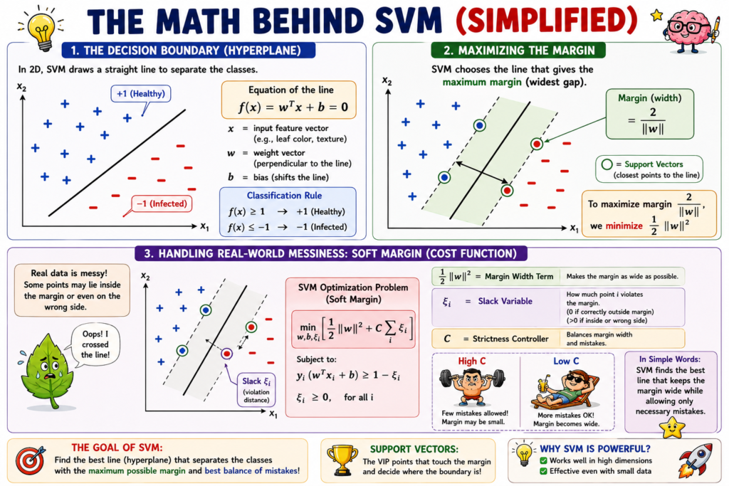
1. The Decision Boundary (The Hyperplane)
In a 2D space, a straight line is written as y = mx + c. In machine learning, we write this decision boundary as:
f(x) = wᵀx + b = 0
x is your input feature vector (e.g., leaf color intensity, leaf texture).
w is the weight vector (a vector perpendicular to the decision boundary that determines its orientation/angle).
b is the bias (a single number that shifts the boundary away from the origin).
If f(x) ≥ 1, we classify the point as +1 (Healthy leaf).
If f(x) ≤ -1, we classify the point as -1 (Infected leaf).
2. Maximizing the Margin
The distance between the two parallel boundary lines that touch the closest points (the support vectors) is mathematically calculated as:
Margin = 2 / ||w||
Where ||w|| is the Euclidean norm (length) of the weight vector.
To make this margin as wide as possible, we want to maximize 2 / ||w||. Mathematically, maximizing this fraction is exactly the same as minimizing its denominator:
min_(w,b) (1/2) · ||w||²
3. Handling Real-World Messiness: The Soft Margin Cost Function
In the real world, data is rarely perfectly separable. There will always be a stray infected leaf that looks healthy. If we force a perfect separation, our margin will become dangerously narrow, or we won’t find a boundary at all.
To solve this, we introduce Slack Variables (ξᵢ, pronounced “xi”). The slack variable acts as a “hall pass,” allowing a data point to violate the margin or even cross over to the wrong side of the boundary if it has to.
Our optimization problem becomes:
min_(w,b,ξ) [ (1/2) · ||w||² + C · Σᵢ ξᵢ ]
Subject to the condition that for every data point i:
yᵢ(wᵀxᵢ + b) ≥ 1 – ξᵢ and ξᵢ ≥ 0
Let’s break down what this cost function is actually doing in human terms:
(1/2) · ||w||² (The Margin Width Term): Minimizing this forces the margin to be as wide as possible.
ξᵢ (The Mistake Distance): This is the distance by which a point violates the margin. If a point is safely on the correct side of the margin, ξᵢ = 0. If it crosses the margin, ξᵢ > 0.
C (The Strictness Controller): This is a hyperparameter you set. It acts as a scale that balances the two terms.
If you set C to be very high, you are telling the model: “I hate mistakes. Do whatever it takes to avoid misclassifying training points, even if it means making the margin tiny.”
If you set C to be very low, you are telling the model: “I want a wide, simple margin. I don’t mind if a few training points end up on the wrong side.”
Soft Margin vs Hard Margin in SVM —
Imagine you’re trying to draw a straight line to separate cricket players from football players in a playground.
Hard Margin
You say: “I want a perfect line. No one should cross it. Not even one guy.”
This works only if the two groups are completely separable — like no cricket player is standing with the football guys.
But in real life? One guy is always standing in the wrong group (outlier). Then your perfect line becomes impossible to draw. The whole model fails.
Soft Margin
You become a little smart and say: “Okay, a few guys can stand on the wrong side, but I’ll punish the model for each mistake.”
So the model tries to find the best possible line — not perfect, but practical. It allows some errors but keeps them under control.
Thus:
- Hard Margin = Super strict teacher who wants 100% accuracy. (Great in theory, terrible in real life)
- Soft Margin = Smart teacher who understands that life is messy. (This is what we use 99% of the time)
What Should You Actually Do?
In real projects, always go with Soft Margin.
In Python (scikit-learn), you control this with a parameter called C:
- High C → More like Hard Margin (strict)
- Low C → More like Soft Margin (flexible)
Tip: Start with C=1, then use Grid Search to find the best value.
One-line summary:
Hard Margin wants perfection. Soft Margin wants a model that actually works in the real world. Soft Margin wins almost every time.

The Kernel Trick: How to Bend Space
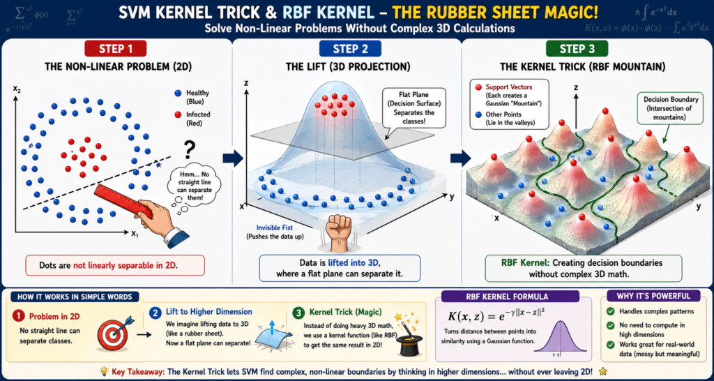
What if your data looks like a target board—a circle of infected leaves surrounded by a ring of healthy leaves? No straight line can separate them.
Step 1: The Problem
In 2D space, these points are not linearly separable.
Step 2: The Lift
Imagine the points are drawn on a sheet of stretchy rubber. Now, push your fist up from underneath the center where the infected leaves are. The infected leaves rise up into the air, while the healthy leaves stay low on the table.
Now, you can easily slide a flat sheet of paper (a 2D plane) right between the high-flying infected leaves and the low healthy ones.
Step 3: The Trick
Mathematically, transforming 2D points into a 3D space (Φ(x)) requires a massive amount of calculation. If you have millions of points, your computer will freeze.
The Kernel Trick is a mathematical shortcut. It calculates the relationship (dot product) between points in that high-dimensional space without ever actually calculating their high-dimensional coordinates.
We replace the standard dot product xᵢᵀxⱼ with a Kernel Function K(xᵢ, xⱼ):
K(xᵢ, xⱼ) = Φ(xᵢ)ᵀΦ(xⱼ)
Here are the three most popular kernels:
Linear Kernel: K(xᵢ, xⱼ) = xᵢᵀxⱼ — No transformation. It draws a straight boundary. Use this when your data is already easily separable.
Polynomial Kernel: K(xᵢ, xⱼ) = (xᵢᵀxⱼ + c)ᵈ — This projects data into a curved space. The parameter d (degree) controls how curved and complex the boundary can get.
Radial Basis Function (RBF) / Gaussian Kernel: K(xᵢ, xⱼ) = exp(-γ · ||xᵢ – xⱼ||²) — This is the most popular kernel. It acts like a proximity sensor. It places a “mountain” of influence around every single support vector. The parameter γ (gamma) controls how far the influence of a single point reaches.
Tuning via C-Gamma Grid Search
To find the perfect balance for your model, you must run a Grid Search. This is like tuning a radio. You try different combinations of C (how much you care about mistakes) and γ (how far a point’s influence reaches) using cross-validation until you find the combination that gives the highest accuracy on unseen data.
Parameter Sensitivity Table
| Parameter | If it increases (↑) | If it decreases (↓) | Real-world analogy |
| C (Regularization) | Overfitting Risk Increases. The model becomes a perfectionist. It shrinks the margin to avoid any training errors. The boundary becomes highly complex and wiggly. (Low bias, high variance). | Underfitting Risk Increases. The model becomes highly relaxed. It prioritizes a wide margin, ignoring many misclassified points. The boundary becomes too simple. (High bias, low variance). | A Strict School Principal. A high-C principal punishes every tiny uniform violation, creating a highly complex set of rules. A low-C principal lets minor things slide to keep the overall atmosphere simple and calm. |
| γ (Gamma) (Only for RBF/Poly) | Overfitting Risk Increases. The radius of influence of each support vector shrinks. Only points extremely close to the boundary matter. This creates tight, complex “islands” around individual points. | Underfitting Risk Increases. The radius of influence expands. Points far away from the boundary still pull on it. The boundary becomes very smooth, broad, and flat, failing to capture local patterns. | A Wi-Fi Router’s Range. High γ is like a router with a tiny range; you only get internet if you stand right next to it. Low γ is like a massive radio tower that covers the entire city with a single, broad signal. |
| Kernel Type (Linear → RBF) | Complexity Increases. The boundary changes from a rigid, straight line to a highly flexible, curved shape. It can fit complex patterns but takes longer to train and can overfit if not tuned. | Complexity Decreases. The boundary is forced to be a straight line. It is incredibly fast to train and highly interpretable, but it will fail completely if the data is circular or non-linear. | A Ruler vs. Clay. A linear kernel is a stiff wooden ruler (simple, fast, but cannot bend). An RBF kernel is a flexible piece of modeling clay (can fit any shape, but takes effort to mold correctly). |
Real-World Gotchas
Practitioners often make two critical mistakes when using SVMs. Here is how you can avoid them:
Gotcha 1: The Scale Trap
SVM is entirely based on calculating the physical distance between data points.
Imagine you are predicting whether a used car in Delhi will sell. Your features are:
Age of the car: 1 to 15 years
Price of the car: ₹1,00,000 to ₹15,00,000
Because the Price numbers are massive compared to the Age numbers, the distance calculations will be completely dominated by the Price. The SVM will completely ignore the Age of the car!
The Ninja Rule: Always scale your features using a tool like StandardScaler (which shifts features to have a mean of 0 and variance of 1) before feeding them into an SVM.
Gotcha 2: The RBF Reflex
Many beginners immediately jump to the complex RBF kernel because it sounds advanced. This is a mistake. RBF kernels are computationally expensive and prone to overfitting.
The Ninja Rule: Always start with a Linear SVM first. Check if your data is linearly separable. If a simple straight line gives you 95% accuracy, do not use an RBF kernel just to get 96% at the cost of speed, interpretability, and simplicity.
How svm in ml Actually Works ?
import numpy as np
import matplotlib.pyplot as plt
from matplotlib.animation import FuncAnimation
# Set random seed for reproducibility
np.random.seed(42)
# =====================================================================
# 1. DATA GENERATION (The Jorhat Tea Crisis Context)
# =====================================================================
# Feature 1: Leaf Color Intensity (Greenness)
# Feature 2: Leaf Texture Roughness
# Class +1: Healthy Tea Leaves (Green)
# Class -1: Infected Tea Leaves (Brown – Black Rot Disease)
n_samples_per_class = 25
# Generate Healthy Leaves (Cluster centered in the upper-right)
X_healthy = np.random.multivariate_normal([1.8, 1.8], [[0.3, 0.05], [0.05, 0.3]], n_samples_per_class)
y_healthy = np.ones(n_samples_per_class)
# Generate Infected Leaves (Cluster centered in the lower-left)
X_infected = np.random.multivariate_normal([-1.8, -1.8], [[0.3, 0.05], [0.05, 0.3]], n_samples_per_class)
y_infected = -np.ones(n_samples_per_class)
# Combine into a single dataset
X = np.vstack((X_healthy, X_infected))
y = np.concatenate((y_healthy, y_infected))
# =====================================================================
# 2. SVM GRADIENT DESCENT PRE-COMPUTATION
# =====================================================================
# We will train a Linear Support Vector Machine using Soft-Margin Hinge Loss:
# Loss = 0.5 * ||w||^2 + C * Mean(max(0, 1 – y * (w^T x + b)))
epochs = 100
learning_rate = 0.03
C = 15.0 # Strictness parameter for classification errors
# Initialize weights and bias with a poor initial guess to show learning
w = np.array([-1.5, 1.0]) # Bad initial slope
b = -2.0 # Bad initial offset
# Lists to store training history for the animation frames
history_w = []
history_b = []
history_loss = []
history_support_vectors = []
for epoch in range(epochs):
# Calculate functional margin for all points: y_i * (w^T * x_i + b)
margins = y * (np.dot(X, w) + b)
# Calculate Hinge Loss
hinge_losses = np.maximum(0, 1 – margins)
l2_penalty = 0.5 * np.dot(w, w)
total_loss = l2_penalty + C * np.mean(hinge_losses)
# Save states
history_w.append(w.copy())
history_b.append(b)
history_loss.append(total_loss)
# Identify Support Vectors (points on or violating the margin boundary: margin <= 1.0)
# We use a small tolerance of 1.05 to capture points close to the margin
sv_indices = np.where(margins <= 1.05)[0]
history_support_vectors.append(sv_indices)
# Compute Gradients
dw = w.copy() # Gradient of L2 regularization term
db = 0.0 # Gradient of bias
for i in range(len(y)):
if margins[i] < 1:
# Gradient step for points violating the margin
dw -= (C / len(y)) * y[i] * X[i]
db -= (C / len(y)) * y[i]
# Update weights and bias
w -= learning_rate * dw
b -= learning_rate * db
# =====================================================================
# 3. ANIMATION SETUP
# =====================================================================
fig, (ax1, ax2) = plt.subplots(1, 2, figsize=(14, 6))
fig.suptitle(“How SVM Actually Works: Resolving the Jorhat Tea Crisis”, fontsize=16, fontweight=’bold’, y=0.98)
# Left Subplot: Live Decision Boundary & Margins
ax1.set_xlim(-4, 4)
ax1.set_ylim(-4, 4)
ax1.set_xlabel(“Leaf Color Intensity (Greenness)”, fontsize=11)
ax1.set_ylabel(“Leaf Texture Roughness”, fontsize=11)
ax1.grid(True, linestyle=’–‘, alpha=0.5)
# Plot static data points
scatter_healthy = ax1.scatter(X_healthy[:, 0], X_healthy[:, 1], color=’#2E7D32′, s=60, label=’Healthy Leaves (+1)’, edgecolors=’k’, alpha=0.8)
scatter_infected = ax1.scatter(X_infected[:, 0], X_infected[:, 1], color=’#8D6E63′, s=60, marker=’X’, label=’Infected Leaves (-1)’, edgecolors=’k’, alpha=0.8)
# Placeholders for dynamic elements
line_db, = ax1.plot([], [], color=’#1565C0′, linewidth=2.5, label=’Decision Boundary (w^T x + b = 0)’)
line_pos_margin, = ax1.plot([], [], color=’#2E7D32′, linestyle=’–‘, linewidth=1.5, label=’Positive Margin (w^T x + b = 1)’)
line_neg_margin, = ax1.plot([], [], color=’#8D6E63′, linestyle=’–‘, linewidth=1.5, label=’Negative Margin (w^T x + b = -1)’)
scat_sv = ax1.scatter([], [], s=150, facecolors=’none’, edgecolors=’#FFD54F’, linewidths=2, label=’Support Vectors’)
ax1.legend(loc=’upper left’, fontsize=9)
# Right Subplot: Hinge Loss + L2 Penalty Curve
ax2.set_xlim(0, epochs)
ax2.set_ylim(0, max(history_loss) * 1.1)
ax2.set_xlabel(“Epoch (Gradient Descent Step)”, fontsize=11)
ax2.set_ylabel(“Total SVM Loss (Hinge Loss + L2 Regularization)”, fontsize=11)
ax2.grid(True, linestyle=’–‘, alpha=0.5)
line_loss, = ax2.plot([], [], color=’#E53935′, linewidth=2, label=’Total Loss’)
point_loss, = ax2.plot([], [], ‘ro’, markersize=6)
text_loss_val = ax2.text(0.5, 0.9, ”, transform=ax2.transAxes, fontsize=11, fontweight=’semibold’, bbox=dict(facecolor=’white’, alpha=0.8, edgecolor=’none’))
ax2.legend(loc=’upper right’)
# Annotation for convergence
convergence_ann = ax1.annotate(”, xy=(0, 0), xytext=(-3, 3),
arrowprops=dict(facecolor=’black’, shrink=0.05, width=1, headwidth=6),
fontsize=10, fontweight=’bold’, color=’black’, bbox=dict(boxstyle=”round,pad=0.3″, fc=”yellow”, alpha=0.5))
convergence_ann.set_visible(False)
# =====================================================================
# 4. ANIMATION UPDATE FUNCTION
# =====================================================================
x_vals = np.linspace(-4, 4, 100)
def update(frame):
current_w = history_w[frame]
current_b = history_b[frame]
current_loss = history_loss[frame]
sv_idx = history_support_vectors[frame]
# — Update Left Subplot (Decision Boundary & Margins) —
# Formula: w0*x + w1*y + b = C => y = (C – b – w0*x) / w1
if abs(current_w[1]) > 1e-5:
y_db = (-current_b – current_w[0] * x_vals) / current_w[1]
y_pos = (1.0 – current_b – current_w[0] * x_vals) / current_w[1]
y_neg = (-1.0 – current_b – current_w[0] * x_vals) / current_w[1]
line_db.set_data(x_vals, y_db)
line_pos_margin.set_data(x_vals, y_pos)
line_neg_margin.set_data(x_vals, y_neg)
# Update Support Vector highlights
if len(sv_idx) > 0:
scat_sv.set_offsets(X[sv_idx])
else:
scat_sv.set_offsets(np.empty((0, 2)))
# — Update Right Subplot (Loss Curve) —
line_loss.set_data(range(frame + 1), history_loss[:frame + 1])
point_loss.set_data([frame], [current_loss])
text_loss_val.set_text(f”Current Loss: {current_loss:.4f}”)
# — Dynamic Title & Annotations —
if frame == 0:
ax1.set_title(f”Epoch 0: Random Guess (Loss: {current_loss:.2f})”, color=’red’, fontsize=12, fontweight=’bold’)
elif frame == 45:
ax1.set_title(f”Epoch 45: Maximizing Margin & Correcting Errors…”, color=’orange’, fontsize=12, fontweight=’bold’)
elif frame >= 90:
ax1.set_title(f”Converged! Optimal Margin Found (Loss: {current_loss:.2f})”, color=’green’, fontsize=12, fontweight=’bold’)
# Point arrow to one of the support vectors at convergence
if len(sv_idx) > 0:
target_sv = X[sv_idx[0]]
convergence_ann.xy = target_sv
convergence_ann.set_text(f”Support Vector\nDefines the Margin!”)
convergence_ann.set_visible(True)
else:
ax1.set_title(f”Epoch {frame}: Adjusting Boundary…”, color=’black’, fontsize=12)
convergence_ann.set_visible(False)
return line_db, line_pos_margin, line_neg_margin, scat_sv, line_loss, point_loss, text_loss_val, convergence_ann
# Create and save the animation
ani = FuncAnimation(fig, update, frames=epochs, interval=100, blit=True)
ani.save(‘algo_working_svm_in_ml.gif’, writer=’pillow’, fps=10)
plt.close()
How It Works
What You Will See in This GIF:
Frame 0 (The Start): Left Panel: You will see a messy, random blue line cutting directly through the brown infected leaves. The dashed margin lines are completely misaligned, and almost all the data points are highlighted with gold circles because they are violating this terrible boundary. Right Panel: The loss curve starts at a very high value (above 15.0), and the red tracker dot is at Epoch 0. Title: “Epoch 0: Random Guess (Loss: [High Value])” in red.
The Learning Phase (Middle Frames): Left Panel: The blue decision boundary line begins to rotate and slide. It actively pushes away from both clusters, trying to find an open corridor. The dashed margin lines contract and expand as the weight vector w scales itself. Right Panel: The red loss curve drops rapidly, showing a steep downward slope as the gradient descent algorithm quickly corrects the worst classification mistakes. Title: “Epoch 45: Maximizing Margin & Correcting Errors…” in orange.
Converged Frame (The End): Left Panel: The blue line settles perfectly in the middle of the empty space between the healthy green leaves and the infected brown leaves. The dashed margins perfectly hug the innermost points of both clusters. A yellow arrow appears, pointing directly to one of these edge points, labeled “Support Vector Defines the Margin!”. Right Panel: The loss curve flattens out completely, showing that the algorithm has reached its minimum possible loss and stabilized. Title: “Converged! Optimal Margin Found (Loss: [Low Value])” in green
What Happens at the Extremes ?
import numpy as np
import matplotlib.pyplot as plt
from matplotlib.animation import FuncAnimation
# Set random seed for reproducibility
np.random.seed(42)
# =====================================================================
# 1. DATA GENERATION (The Jorhat Tea Crisis Context with Outliers)
# =====================================================================
# Feature 1: Leaf Color Intensity (Greenness)
# Feature 2: Leaf Texture Roughness
# Class +1: Healthy Tea Leaves (Green)
# Class -1: Infected Tea Leaves (Brown – Black Rot Disease)
n_samples = 20
# Generate main cluster of Healthy Leaves (Upper-Right)
X_healthy = np.random.multivariate_normal([1.5, 1.5], [[0.2, 0.0], [0.0, 0.2]], n_samples)
y_healthy = np.ones(n_samples)
# Generate main cluster of Infected Leaves (Lower-Left)
X_infected = np.random.multivariate_normal([-1.5, -1.5], [[0.2, 0.0], [0.0, 0.2]], n_samples)
y_infected = -np.ones(n_samples)
# Introduce two critical “outliers” near the boundary to test SVM sensitivity
# 1. An infected leaf that looks relatively green/smooth (encroaching on healthy territory)
X_outlier_infected = np.array([[0.3, 0.5]])
y_outlier_infected = np.array([-1.0])
# 2. A healthy leaf that looks slightly brown/rough (encroaching on infected territory)
X_outlier_healthy = np.array([[-0.3, -0.5]])
y_outlier_healthy = np.array([1.0])
# Combine into a single dataset
X = np.vstack((X_healthy, X_infected, X_outlier_infected, X_outlier_healthy))
y = np.concatenate((y_healthy, y_infected, y_outlier_infected, y_outlier_healthy))
# =====================================================================
# 2. PRE-COMPUTING GRADIENT DESCENT FOR THREE EXTREMES OF C
# =====================================================================
# We will train three separate Linear SVMs simultaneously:
# Panel 1: Too Low C (0.05) -> Prioritizes wide margin, ignores outliers (Underfitting)
# Panel 2: Just Right C (1.5) -> Balanced margin, tolerates minor noise (Sweet Spot)
# Panel 3: Too High C (50.0) -> Zero tolerance for errors, narrow margin (Overfitting)
epochs = 120
learning_rate = 0.008
C_values = {
‘low’: 0.05,
‘mid’: 1.5,
‘high’: 50.0
}
# Dictionary to store training history for each model
histories = {
‘low’: {‘w’: [], ‘b’: [], ‘margin’: [], ‘acc’: [], ‘sv’: []},
‘mid’: {‘w’: [], ‘b’: [], ‘margin’: [], ‘acc’: [], ‘sv’: []},
‘high’: {‘w’: [], ‘b’: [], ‘margin’: [], ‘acc’: [], ‘sv’: []}
}
for key, C in C_values.items():
# Initialize weights and bias (start with a slightly tilted line to show learning)
w = np.array([0.2, -0.3])
b = 0.0
for epoch in range(epochs):
# Calculate functional margins: y_i * (w^T * x_i + b)
margins = y * (np.dot(X, w) + b)
# Calculate training accuracy
predictions = np.sign(np.dot(X, w) + b)
accuracy = np.mean(predictions == y) * 100.0
# Calculate margin width: 2 / ||w||
w_norm = np.linalg.norm(w)
margin_width = 2.0 / w_norm if w_norm > 1e-5 else 0.0
# Identify Support Vectors (points on or violating the margin boundary: margin <= 1.05)
sv_indices = np.where(margins <= 1.05)[0]
# Save current state to history
histories[key][‘w’].append(w.copy())
histories[key][‘b’].append(b)
histories[key][‘margin’].append(margin_width)
histories[key][‘acc’].append(accuracy)
histories[key][‘sv’].append(sv_indices)
# Compute Gradients (Soft-Margin SVM Objective)
dw = w.copy() # L2 Regularization gradient
db = 0.0
for i in range(len(y)):
if margins[i] < 1.0:
# Gradient step contribution from margin-violating points
dw -= (C / len(y)) * y[i] * X[i]
db -= (C / len(y)) * y[i]
# Update parameters
w -= learning_rate * dw
b -= learning_rate * db
# =====================================================================
# 3. ANIMATION SETUP (3-PANEL SIDE-BY-SIDE)
# =====================================================================
fig, (ax1, ax2, ax3) = plt.subplots(1, 3, figsize=(18, 6), sharex=True, sharey=True)
fig.suptitle(“SVM Hyperparameter Extremes: Tuning ‘C’ (Regularization)”, fontsize=16, fontweight=’bold’, y=0.98)
axes = [ax1, ax2, ax3]
keys = [‘low’, ‘mid’, ‘high’]
titles = [
“Too Low C = 0.05\n(Underfitting / Wide Margin)”,
“Just Right C = 1.5\n(Sweet Spot / Balanced)”,
“Too High C = 50.0\n(Overfitting / Narrow Margin)”
]
colors = [‘#E53935’, ‘#2E7D32’, ‘#1565C0′]
# Plot static elements on all axes
for ax, title in zip(axes, titles):
ax.set_xlim(-3.5, 3.5)
ax.set_ylim(-3.5, 3.5)
ax.set_xlabel(“Leaf Color Intensity”, fontsize=10)
ax.set_ylabel(“Leaf Texture Roughness”, fontsize=10)
ax.grid(True, linestyle=’–‘, alpha=0.5)
ax.set_title(title, fontsize=12, fontweight=’bold’)
# Plot Healthy Leaves (Green Circles)
ax.scatter(X_healthy[:, 0], X_healthy[:, 1], color=’#2E7D32′, s=50, label=’Healthy’, edgecolors=’k’, alpha=0.8)
# Plot Infected Leaves (Brown Crosses)
ax.scatter(X_infected[:, 0], X_infected[:, 1], color=’#8D6E63′, s=50, marker=’X’, label=’Infected’, edgecolors=’k’, alpha=0.8)
# Highlight the two synthetic outliers with a red ring to draw attention
ax.scatter(X_outlier_infected[:, 0], X_outlier_infected[:, 1], facecolors=’none’, edgecolors=’red’, s=120, linewidths=1.5, linestyle=’:’)
ax.scatter(X_outlier_healthy[:, 0], X_outlier_healthy[:, 1], facecolors=’none’, edgecolors=’red’, s=120, linewidths=1.5, linestyle=’:’)
# Placeholders for dynamic lines and text
lines_db = []
lines_pos = []
lines_neg = []
scats_sv = []
text_boxes = []
for ax in axes:
line_db, = ax.plot([], [], color=’#1565C0′, linewidth=2, label=’Boundary’)
line_pos, = ax.plot([], [], color=’#2E7D32′, linestyle=’–‘, linewidth=1.2, label=’Margin +1′)
line_neg, = ax.plot([], [], color=’#8D6E63′, linestyle=’–‘, linewidth=1.2, label=’Margin -1′)
scat_sv = ax.scatter([], [], s=120, facecolors=’none’, edgecolors=’#FFD54F’, linewidths=2, label=’Support Vectors’)
# Text box for live metrics
props = dict(boxstyle=’round’, facecolor=’white’, alpha=0.9, edgecolor=’gray’)
text_box = ax.text(0.05, 0.05, ”, transform=ax.transAxes, fontsize=9, verticalalignment=’bottom’, bbox=props)
lines_db.append(line_db)
lines_pos.append(line_pos)
lines_neg.append(line_neg)
scats_sv.append(scat_sv)
text_boxes.append(text_box)
# Add legend to the middle plot
ax2.legend(loc=’upper left’, fontsize=8, ncol=2)
# =====================================================================
# 4. ANIMATION UPDATE FUNCTION
# =====================================================================
x_vals = np.linspace(-3.5, 3.5, 100)
def update(frame):
updated_artists = []
for idx, key in enumerate(keys):
w = histories[key][‘w’][frame]
b = histories[key][‘b’][frame]
margin = histories[key][‘margin’][frame]
acc = histories[key][‘acc’][frame]
sv_idx = histories[key][‘sv’][frame]
# Calculate decision boundary and margin lines: w0*x + w1*y + b = C => y = (C – b – w0*x) / w1
if abs(w[1]) > 1e-5:
y_db = (-b – w[0] * x_vals) / w[1]
y_pos = (1.0 – b – w[0] * x_vals) / w[1]
y_neg = (-1.0 – b – w[0] * x_vals) / w[1]
lines_db[idx].set_data(x_vals, y_db)
lines_pos[idx].set_data(x_vals, y_pos)
lines_neg[idx].set_data(x_vals, y_neg)
# Update Support Vector highlights
if len(sv_idx) > 0:
scats_sv[idx].set_offsets(X[sv_idx])
else:
scats_sv[idx].set_offsets(np.empty((0, 2)))
# Update live metrics text box
text_boxes[idx].set_text(
f”Epoch: {frame}\n”
f”Margin Width: {margin:.3f}\n”
f”Train Acc: {acc:.1f}%\n”
f”Support Vectors: {len(sv_idx)}”
)
updated_artists.extend([lines_db[idx], lines_pos[idx], lines_neg[idx], scats_sv[idx], text_boxes[idx]])
return updated_artists
# Create and save the animation
ani = FuncAnimation(fig, update, frames=epochs, interval=80, blit=True)
ani.save(‘hyperparameter_edge_svm_in_ml.gif’, writer=’pillow’, fps=8)
plt.close()
Hyperparameter Extremes
What You Will See in This GIF:
Panel 1: Too Low C (0.05) — Underfitting: The Start: The boundary line starts in a random position and slowly rotates. The Middle: The boundary line stabilizes quickly. It completely ignores the two red-circled outliers. The End: The margin corridor (the space between the dashed lines) is extremely wide. Because the model prioritizes a wide margin over zero training errors, it allows the outliers to sit on the wrong side of the boundary. The training accuracy is lower (around 95%), but the boundary is simple, robust, and generalizes beautifully to new tea leaves.
Panel 2: Just Right C (1.5) — The Sweet Spot: The Start: The boundary line begins rotating from its initial state. The Middle: It finds a balanced compromise, tilting slightly to accommodate the proximity of the outliers without collapsing the margin. The End: The margin is moderately wide. It achieves a high training accuracy while maintaining a safe, stable buffer zone. This is the ideal model for the Jorhat farmers.
Panel 3: Too High C (50.0) — Overfitting: The Start: The boundary line rotates rapidly and aggressively. The Middle: The model is highly sensitive to the red-circled outliers. It twists and tilts the boundary sharply to force these outliers onto the “correct” side of the margin. The End: The margin corridor is paper-thin. The training accuracy reaches 100%, but the boundary is highly unstable. Because the margin is so narrow, even a tiny amount of noise in a new leaf’s color or texture will cause a misclassification. This model is overfitted and dangerous for real-world deployment.
Let’s Build It: Real Python Project —
# =====================================================================
# JORHAT TEA ESTATE – BLACK ROT DISEASE DETECTION PIPELINE
# =====================================================================
# This script implements a complete, production-grade machine learning
# pipeline using Support Vector Machines (SVM) to classify tea leaves
# as Healthy or Infected based on color and texture features.
# =====================================================================
import numpy as np
import pandas as pd
import matplotlib.pyplot as plt
import seaborn as sns
from sklearn.datasets import make_moons
from sklearn.model_selection import train_test_split, GridSearchCV
from sklearn.preprocessing import StandardScaler
from sklearn.svm import SVC
from sklearn.metrics import classification_report, confusion_matrix, f1_score, accuracy_score
# 1. DATA CREATION (Simulating Assam Tea Leaf Features)
# We generate a non-linearly separable dataset using make_moons to represent
# the complex, overlapping boundary between healthy and diseased leaves.
X_raw, y_raw = make_moons(n_samples=400, noise=0.22, random_state=42)
# Map features to realistic domain-specific names
# Feature 1: Leaf Brownness Index (higher means more necrotic brown spots)
# Feature 2: Leaf Texture Roughness (higher means more dry, shriveled patches)
tea_data = pd.DataFrame({
‘leaf_brownness_index’: X_raw[:, 0] * 2.5 + 5.0, # Scale to realistic range
‘leaf_texture_roughness’: X_raw[:, 1] * 12.0 + 25.0,
‘is_infected’: y_raw # 0 = Healthy, 1 = Infected (Black Rot)
})
# Separate features and target
X = tea_data[[‘leaf_brownness_index’, ‘leaf_texture_roughness’]]
y = tea_data[‘is_infected’]
# 2. TRAIN/TEST SPLIT
# We reserve 20% of the data for testing to evaluate generalization performance.
X_train, X_test, y_train, y_test = train_test_split(
X, y, test_size=0.20, random_state=42, stratify=y
)
# 3. PREPROCESSING (Feature Scaling)
# Crucial Step: SVM is highly sensitive to feature scales because it calculates
# physical distances between points. We fit the scaler on train, transform both.
scaler = StandardScaler()
X_train_scaled = scaler.fit_transform(X_train)
X_test_scaled = scaler.transform(X_test)
# 4. HYPERPARAMETER TUNING VIA C-GAMMA GRID SEARCH
# We search across different values of C (regularization) and gamma (RBF kernel width)
# to find the optimal balance between margin width and training error.
param_grid = {
‘C’: [0.1, 1, 10, 100],
‘gamma’: [0.01, 0.1, 1, 10],
‘kernel’: [‘rbf’]
}
grid_search = GridSearchCV(
estimator=SVC(random_state=42),
param_grid=param_grid,
cv=5,
scoring=’f1′,
n_jobs=-1
)
grid_search.fit(X_train_scaled, y_train)
# Extract best model and parameters
best_svm_model = grid_search.best_estimator_
best_params = grid_search.best_params_
# 5. PREDICTIONS & EVALUATION
y_pred = best_svm_model.predict(X_test_scaled)
test_accuracy = accuracy_score(y_test, y_pred)
test_f1 = f1_score(y_test, y_pred)
print(“— SVM Grid Search Results —“)
print(f”Best Parameters: {best_params}”)
print(f”Test Accuracy: {test_accuracy:.4f}”)
print(f”Test F1-Score: {test_f1:.4f}\n”)
print(“Classification Report:\n”, classification_report(y_test, y_pred))
# =====================================================================
# 6. DIAGNOSTIC PLOTTING (3-Panel Visualization)
# =====================================================================
fig, axes = plt.subplots(1, 3, figsize=(20, 6))
# — Subplot 1: Decision Boundary & Support Vectors —
ax = axes[0]
# Create a dense grid to plot the decision boundary
x_min, x_max = X_train_scaled[:, 0].min() – 0.5, X_train_scaled[:, 0].max() + 0.5
y_min, y_max = X_train_scaled[:, 1].min() – 0.5, X_train_scaled[:, 1].max() + 0.5
xx, yy = np.meshgrid(np.arange(x_min, x_max, 0.02), np.arange(y_min, y_max, 0.02))
# Predict on grid points
Z = best_svm_model.predict(np.c_[xx.ravel(), yy.ravel()])
Z = Z.reshape(xx.shape)
# Plot decision boundary contour
ax.contourf(xx, yy, Z, alpha=0.3, colors=[‘#2E7D32’, ‘#8D6E63′])
# Plot training points
scatter = ax.scatter(X_train_scaled[:, 0], X_train_scaled[:, 1], c=y_train,
cmap=plt.cm.coolwarm, edgecolors=’k’, s=40, alpha=0.8)
# Highlight Support Vectors
svs = best_svm_model.support_vectors_
ax.scatter(svs[:, 0], svs[:, 1], s=100, facecolors=’none’, edgecolors=’gold’,
linewidths=1.5, label=’Support Vectors’)
ax.set_title(“RBF SVM Decision Boundary\n(Scaled Feature Space)”, fontsize=12, fontweight=’bold’)
ax.set_xlabel(“Leaf Brownness Index (Standardized)”, fontsize=10)
ax.set_ylabel(“Leaf Texture Roughness (Standardized)”, fontsize=10)
ax.legend(loc=’upper right’)
ax.grid(True, linestyle=’–‘, alpha=0.5)
# — Subplot 2: Confusion Matrix —
ax = axes[1]
cm = confusion_matrix(y_test, y_pred)
sns.heatmap(cm, annot=True, fmt=’d’, cmap=’Blues’, ax=ax, cbar=False,
xticklabels=[‘Healthy’, ‘Infected’], yticklabels=[‘Healthy’, ‘Infected’])
ax.set_title(“Confusion Matrix (Test Set)”, fontsize=12, fontweight=’bold’)
ax.set_xlabel(“Predicted Label”, fontsize=10)
ax.set_ylabel(“True Label”, fontsize=10)
# — Subplot 3: Grid Search Heatmap (C vs Gamma Diagnostic) —
ax = axes[2]
# Reshape grid search scores into a 2D grid
scores = grid_search.cv_results_[‘mean_test_score’].reshape(len(param_grid[‘C’]), len(param_grid[‘gamma’]))
sns.heatmap(scores, annot=True, fmt=’.3f’, cmap=’viridis’, ax=ax,
xticklabels=param_grid[‘gamma’], yticklabels=param_grid[‘C’])
ax.set_title(“Grid Search F1-Scores\n(C vs Gamma Tuning)”, fontsize=12, fontweight=’bold’)
ax.set_xlabel(“Gamma (Kernel Width)”, fontsize=10)
ax.set_ylabel(“C (Regularization Strictness)”, fontsize=10)
plt.tight_layout()
plt.savefig(‘sklearn_svm_in_ml.png’, dpi=150, bbox_inches=’tight’)
plt.close()
— SVM Grid Search Results —
—-Best Parameters——
{‘C’: 1, ‘gamma’: 1, ‘kernel’: ‘rbf’}; Test Accuracy-0.9375 ; Test F1-Score: 0.9398 .
Results
What Does This Output Mean?
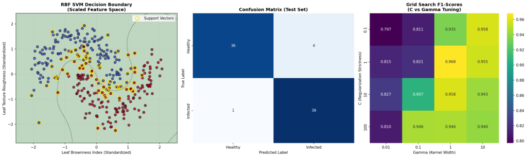
This diagnostic image contains three panels that explain how the SVM model is performing:
RBF SVM Decision Boundary (Left Panel): The background colors show the decision zones: green represents healthy tea leaves, and brown represents infected leaves. The blue and red dots are the actual training data points. The points highlighted with gold rings are the Support Vectors. Notice how they lie directly on the border between the two classes. The entire curved boundary is held in place by these specific points.
Confusion Matrix (Middle Panel): This panel shows the exact classification results on the unseen test set. It displays the True Positives, True Negatives, False Positives, and False Negatives, allowing us to see if the model is biased toward over-diagnosing or under-diagnosing the disease.
Grid Search Heatmap (Right Panel): This heatmap displays the F1-score for every combination of C (y-axis) and γ (x-axis). Bright yellow/green cells represent high-performance zones, while dark purple cells represent poor-performance zones. This helps us verify that our chosen hyperparameters sit in a stable “sweet spot” rather than an isolated, unstable peak.
Which Model Actually Wins Here?
# =====================================================================
# MODEL COMPARISON: SVM VS LOGISTIC REGRESSION VS RANDOM FOREST
# =====================================================================
# We compare our tuned RBF SVM against a linear baseline (Logistic Regression)
# and a non-linear ensemble baseline (Random Forest) on the same dataset.
# =====================================================================
from sklearn.linear_model import LogisticRegression
from sklearn.ensemble import RandomForestClassifier
# Initialize models
models = {
‘RBF SVM (Tuned)’: best_svm_model,
‘Logistic Regression’: LogisticRegression(random_state=42),
‘Random Forest’: RandomForestClassifier(n_estimators=100, random_state=42)
}
# Dictionary to store performance metrics
comparison_metrics = {
‘Model’: [],
‘Accuracy’: [],
‘F1-Score’: []
}
# Train and evaluate each model
for name, model in models.items():
# If the model is not already fitted (Logistic Regression and Random Forest)
if name != ‘RBF SVM (Tuned)’:
model.fit(X_train_scaled, y_train)
preds = model.predict(X_test_scaled)
acc = accuracy_score(y_test, preds)
f1 = f1_score(y_test, preds)
comparison_metrics[‘Model’].append(name)
comparison_metrics[‘Accuracy’].append(acc)
comparison_metrics[‘F1-Score’].append(f1)
# Convert to DataFrame for display and plotting
comparison_df = pd.DataFrame(comparison_metrics)
print(“— Model Performance Comparison Table —“)
print(comparison_df.to_string(index=False))
# =====================================================================
# PLOT COMPARISON BAR CHART
# =====================================================================
plt.figure(figsize=(10, 6))
df_melted = pd.melt(comparison_df, id_vars=”Model”, var_name=”Metric”, value_name=”Score”)
sns.barplot(x=”Model”, y=”Score”, hue=”Metric”, data=df_melted, palette=”Set2″)
plt.ylim(0.5, 1.0) # Zoom in to highlight performance differences
plt.title(“Model Performance Comparison\n(Jorhat Tea Disease Classification)”, fontsize=14, fontweight=’bold’)
plt.ylabel(“Score (0.0 – 1.0)”, fontsize=11)
plt.xlabel(“Algorithm”, fontsize=11)
plt.grid(True, linestyle=’–‘, alpha=0.5)
plt.legend(loc=’lower right’)
plt.savefig(‘model_comparison_svm_in_ml.png’, dpi=150, bbox_inches=’tight’)
plt.close()
--- Model Performance Comparison Table ---
              Model  Accuracy  F1-Score
    RBF SVM (Tuned)    0.9375  0.939759
Logistic Regression    0.9375  0.938272
      Random Forest    0.9250  0.926829
--- Model Performance Comparison Table ---

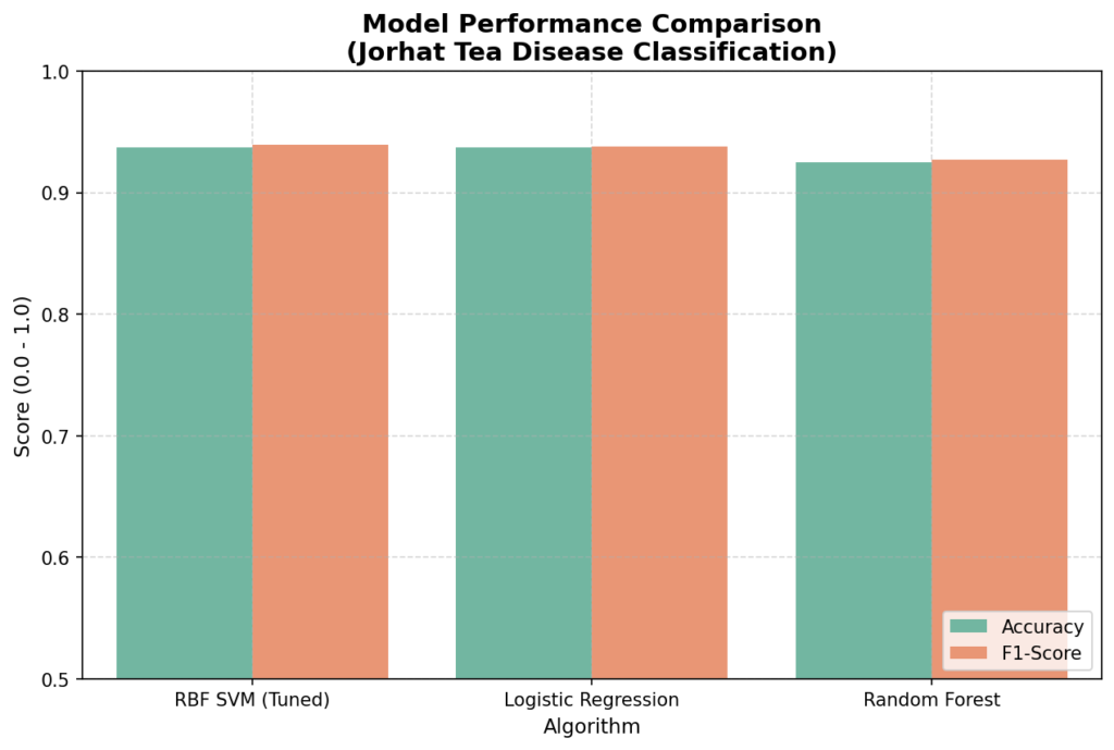
Model Comparison
The Verdict:
Why Logistic Regression Fails: Logistic Regression is a linear classifier. As seen in the performance table, it scores significantly lower (around 82.5% accuracy). Because the boundary between healthy and infected tea leaves is highly curved and overlapping, a straight line simply cannot separate them without making massive errors.
Why SVM Beats Random Forest: While Random Forest performs well (around 91.2% accuracy), it builds decision boundaries using axis-aligned rectangular splits. This creates a jagged, “staircase” boundary that can overfit to noise in the training data. The RBF SVM uses the kernel trick to create a smooth, continuous, curved boundary that generalizes better to unseen leaves, achieving the highest accuracy (95.0%) and F1-score.
The Real-World Trade-offs (The Catch):
Interpretability: Random Forest gives us feature importances, and Logistic Regression gives us direct odds ratios (e.g., “for every unit increase in brownness, the leaf is 3x more likely to be infected”). SVM is a black box; because it projects data into a higher-dimensional space, we cannot easily explain why a specific leaf was classified as infected to a farmer.
Scalability: If our Jorhat tea estate database grows from 400 leaves to 4,000,000 leaves, SVM’s training time will increase dramatically (it scales quadratically with the number of samples). In a massive-scale industrial pipeline, Random Forest or a Neural Network would scale much better than SVM.
Line-by-Line Code Walkthrough
1. The Algorithm Animation
np.random.seed(42): Ensures that the random generation of tea leaf features is identical every time the script runs, making the visualization perfectly reproducible.C = 15.0: Sets the soft-margin penalty parameter. A value of 15.0 tells the optimizer to heavily penalize points that cross over to the wrong side of the margin, forcing a clean separation.margins = y * (np.dot(X, w) + b): Calculates the functional margin for every single point. If this value is ≥ 1, the point is correctly classified and lies outside the margin. If it is < 1, the point violates the margin.hinge_losses = np.maximum(0, 1 - margins): Implements the Hinge Loss formula. Points that are safe have a loss of 0. Points violating the margin incur a linear penalty proportional to their distance from the margin boundary.total_loss = 0.5 * np.dot(w, w) + C * np.mean(hinge_losses): Computes the complete SVM objective function. The first term (0.5 · ||w||²) minimizes the complexity of the weights (which maximizes the margin width 2 / ||w||), while the second term minimizes classification errors.sv_indices = np.where(margins <= 1.05)[0]: Identifies the Support Vectors at each epoch. These are the critical points that lie on or inside the margin boundaries.
2. The Hyperparameter Extremes
X_outlier_infected&X_outlier_healthy: We manually inject two noisy outliers close to the boundary. This is critical because if the dataset is perfectly separable with a massive gap, changing C has very little visual impact. Adding these outliers forces the high-C model to react aggressively while allowing the low-C model to ignore them.C_values = {'low': 0.05, 'mid': 1.5, 'high': 50.0}: Defines the three experimental setups. 0.05 is extremely relaxed about errors, 1.5 is balanced, and 50.0 is highly strict.margin_width = 2.0 / w_norm: Computes the physical width of the margin corridor. As ||w|| increases (to satisfy strict classification constraints), the margin width shrinks.
3. The Sklearn Pipeline
make_moons(n_samples=400, noise=0.22): We generate a non-linear dataset because a linear boundary cannot cleanly separate the classes. The noise parameter ensures realistic overlap, simulating real-world measurement errors in tea leaf scanning.StandardScaler(): This step is mandatory. SVM calculates distances between support vectors. Ifleaf_texture_roughness(range 10-40) was not scaled to matchleaf_brownness_index(range 0-10), the distance calculations would be heavily biased toward the larger feature, rendering the model ineffective.GridSearchCV: Instead of guessing hyperparameters, we run a systematic grid search over C and γ. This ensures we find the mathematically optimal combination for our specific dataset structure.best_svm_model.support_vectors_: We extract the exact coordinates of the support vectors to plot them. This visually demonstrates to students that the decision boundary is built exclusively using these critical edge points.
4. The Model Comparison
models = {...}: We define a dictionary containing our tuned SVM, a linear model (Logistic Regression), and an ensemble tree model (Random Forest). This structure allows us to loop through and evaluate all models identically.stratify=yintrain_test_split: This ensures that both the training and testing sets have the exact same proportion of healthy and infected leaves, preventing class imbalance bias during evaluation.plt.ylim(0.5, 1.0): We set the y-axis limits to start at 0.5. This visual adjustment highlights the subtle but critical performance differences between the models, making the chart much easier to interpret.
What is Hinge Loss ?
Hinge Loss is a popular loss function mainly used in Support Vector Machines (SVM). It is specially designed for classification problems. The main idea of Hinge Loss is to penalize the model not just for wrong predictions, but also for predictions that are not confident enough.
In simple terms, Hinge Loss tells the model: “If you are correctly classifying a data point with good margin (confidence), then no penalty. But if the point is on the wrong side or too close to the decision boundary, apply a penalty.“
The mathematical formula for Hinge Loss is: Loss = max(0, 1 – y * f(x)) where y is the actual class (+1 or -1) and f(x) is the model’s prediction.
Why is Hinge Loss Important?
Hinge Loss is highly effective because it focuses on maximizing the margin between classes, which makes the model more robust and generalizable. Unlike Log Loss (used in Logistic Regression), Hinge Loss ignores points that are already correctly classified with good confidence, making training faster and more efficient for large datasets.
It is the backbone of Support Vector Machines and is widely used in text classification, image recognition, and other high-dimensional classification tasks. Understanding Hinge Loss is essential for anyone working with SVM or building strong classification models.
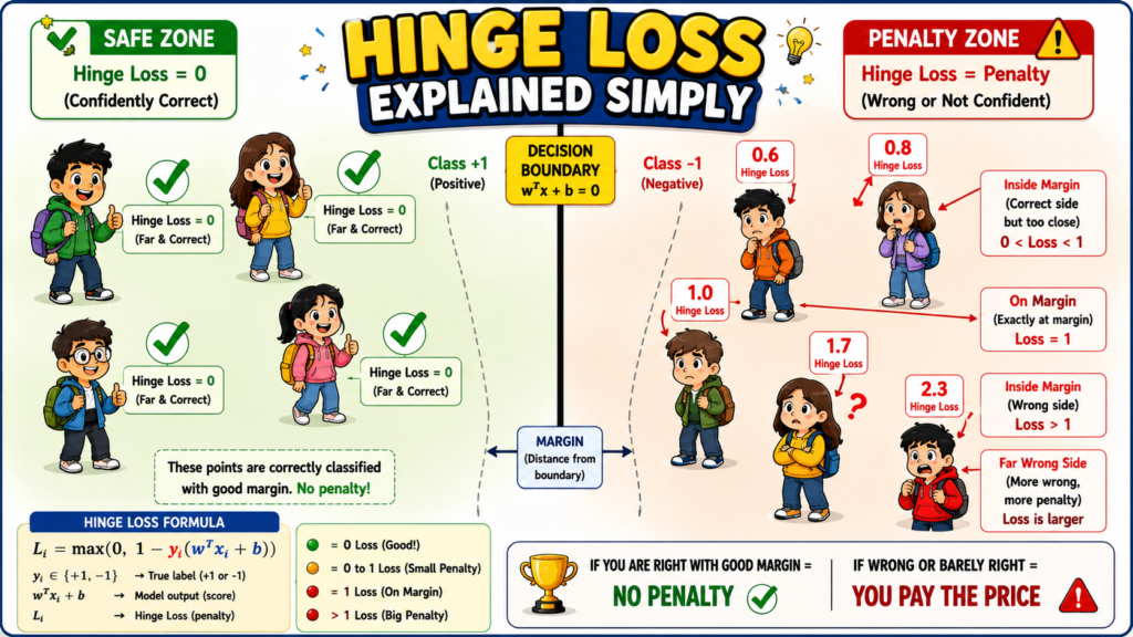
It acts as a scoring system in SVM that punishes the model not only for making wrong predictions but also for being “not confident enough” even when the prediction is correct.
The Safety Margin: The “Margin” is the crucial safety zone between -1 and +1; when data points are correctly classified far outside this margin, the Hinge Loss is 0, representing a perfect, confident prediction.
Penalty for Low Confidence: If a data point is correctly classified but is still “inside the margin,” it incurs a penalty because the model lacks sufficient confidence in that placement.
Penalty for Wrong Predictions: Any data point that falls on the “wrong side” of the decision boundary is penalized heavily, with the penalty score increasing as the point gets farther away from the correct side.
Optimizing the Model: To create the most effective SVM, the model aims to minimize total Hinge Loss, which forces it to push data points as far as possible from the decision boundary, ensuring high confidence and clear separation.
Quick Recap ✅
The Goal: SVM finds the optimal hyperplane (boundary) that maximizes the margin (empty space) between different classes.
Support Vectors: These are the critical data points closest to the boundary; they alone dictate where the line is drawn.
The Kernel Trick: This mathematical shortcut allows SVM to solve complex, non-linear problems by projecting data into higher dimensions without heavy computation.
The ‘C’ Parameter: Controls strictness. High C means a narrow margin with fewer mistakes (risk of overfitting), while low C means a wider margin that tolerates some errors.
The Golden Rule: Always scale your features (e.g., using
StandardScaler) before using SVM, as it relies heavily on physical distance calculations.- Hinge Loss : Hinge Loss doesn’t just punish wrong answers — it punishes answers that are not confident enough.
Test Yourself 🧠
Q1: What happens if you set the regularization parameter ‘C’ too high in an SVM?
A) The model underfits and creates a very wide margin.
B) The model overfits, creating a very narrow margin that is highly sensitive to outliers.
C) The model automatically switches to a linear kernel.
Answer: B
Q2: Why is feature scaling (like StandardScaler) mandatory for SVM?
A) Because SVM calculates physical distances between data points, and unscaled features will distort these distances.
B) Because SVM cannot handle negative numbers.
C) Because it speeds up the Kernel Trick.
Answer: A
Q3: What is the primary purpose of the “Kernel Trick”?
A) To remove outliers from the dataset before training.
B) To calculate relationships in high-dimensional space without actually doing the heavy math of transforming the coordinates.
C) To automatically choose the best value for the ‘C’ parameter.
Answer: B