Imagine you bought a high-end, expensive GPU, cranked up your batch size, and turned on mixed precision. Your VRAM is completely full—yet when you check the profiler, training feels sluggish.
Why? Because in standard PyTorch Eager Mode, your GPU constantly stops and waits. It performs a tiny piece of work, pauses for Python, launches a CUDA kernel, pauses again, and launches the next one.
Think of it like hiring 1,000 lightning-fast factory workers, but giving them instructions one by one:
“Pick up this box.” (Wait.)
“Move it there.” (Wait.)
“Open it.” (Wait.)
The workers (your GPU hardware) are blazing fast, but the instruction system (Python and kernel launching overhead) is bottlenecking everything.
Enter torch.compile(): Fixing the Bottleneck
This is exactly what PyTorch torch.compile() is built to solve.
Instead of running every single math operation independently, torch.compile() looks at a big block of your code all at once. It optimizes the entire chain, fuses compatible operations together, and compiles them directly into high-performance hardware code. On GPUs, this creates specialized Triton kernels via TorchInductor.
And best of all, enabling it can be as simple as adding a single line to your model:
model.compile()
# or
compiled_model = torch.compile(model)
That one line looks simple, but under the hood, an entire compiler pipeline is spinning up. Let’s open the hood and see how it actually works.
What Is Normal PyTorch Eager Execution?
To understand why PyTorch optimization matters, let’s look at how PyTorch executes code by default. This is known as eager execution.
Consider this simple Python function:
def transform(x, bias):
    x = x + bias
    x = x * 0.5
    x = torch.relu(x)
    return x
To a developer, this looks like one quick, unified transformation. But under the hood in eager mode, your GPU doesn’t see it that way.
How the GPU Sees Eager Execution?
Instead of handling everything at once, standard PyTorch executes each line independently. The GPU breaks this down into three separate hardware instructions called CUDA kernels:
Kernel 1: Add the bias to
x.Kernel 2: Multiply the result by
0.5.Kernel 3: Apply the ReLU activation function.
The Two Major Bottlenecks of Eager Mode:
1. Kernel Launch Overhead: Every single time the Python interpreter tells the GPU to run an operation, it causes a brief pause (overhead) while launching a new CUDA kernel. Launching three separate kernels means three separate pauses.
2. The VRAM Traffic Bottleneck: Modern GPUs are lightning-fast at raw math (arithmetic). The real bottleneck is moving data back and forth. In eager mode, intermediate data must constantly bounce between high-latency global GPU memory (VRAM) and the GPU’s internal compute units:
VRAM → GPU Compute → VRAM (After Step 1)
VRAM → GPU Compute → VRAM (After Step 2)
VRAM → GPU Compute → VRAM (After Step 3)
Think of it like a chef taking an ingredient out of the refrigerator, cutting it, putting it back into the fridge, taking it out again for the next step, and repeating. It wastes enormous amounts of time.
Enter torch.compile():
Instead of treating every line as an isolated command, torch.compile() looks at the entire chain of operations together. It analyzes how data flows from one step to the next, sets the stage for kernel fusion, and feeds your GPU efficiently.
What Actually Happens Inside torch.compile()?
When you call torch.compile(), your code doesn’t just magically run faster. It travels through a powerful compiler pipeline that reorganizes how your GPU executes instructions.
Here is the exact pipeline flow:
Your PyTorch Code
        ↓
   TorchDynamo       (Captures operations into an FX Graph)
        ↓
   AOTAutograd       (Handles training forward & backward passes)
        ↓
  TorchInductor      (The default backend generating fast code)
        ↓
   Triton Kernels    (Custom high-performance GPU code)
        ↓
       GPU           (Lightning-fast execution)
Let us break down each layer in simple terms.
Step 1: TorchDynamo (Capturing Python Execution)
Normally, PyTorch executes operations one by one as Python commands. TorchDynamo sits in the background, watches your Python code run, and captures tensor operations into an FX Graph.
Suppose your function looks like this:
x = torch.sin(x)
y = torch.cos(x)
z = x + y
Instead of treating sin, cos, and addition as three separate, isolated commands, Dynamo captures them as a connected graph.
The Big Picture: The compiler now sees that
xfeeds intosin, which feeds into subsequent math. It can look at the whole chain and ask: “Can we optimize or fuse these operations together?”Caching: PyTorch caches the compiled version so it can reuse it instantly next time.
The Concept of “Guards”
To keep things safe, the compiler makes strict assumptions about your tensors. For example:
Input must be a Tensor
Data type:
float32Device:
cudaShape:
32 × 1024
PyTorch records these conditions as Guards.
When your function runs again, the guards are checked. If valid, it reuses the fast compiled code.
If your input shape or data type changes, a guard fails. When a guard fails, PyTorch is forced to trigger a recompilation (which causes a brief pause).
Step 2: AOTAutograd (Making Training Fast)
Inference (making predictions) is only half the battle. Deep learning training requires two major phases:
Forward pass (calculating predictions and loss)
Backward pass (calculating gradients via backpropagation)
Normal Eager Mode: Builds the backward computation graph dynamically on the fly every single time.
AOTAutograd (Ahead-Of-Time Autograd): Gives the compiler access to graph representations for both the forward and backward passes before execution.
This allows compiler optimizations to wrap around the entire training loop—which is why torch.compile() speeds up training just as effectively as inference.
Step 3: TorchInductor (Generating Optimized Code)
TorchInductor is the default compiler backend used under the hood by torch.compile().
You can see this explicitly in the API if you want:
torch.compile(model, backend="inductor")
(You normally don’t need to type backend="inductor" because PyTorch already sets it as the default.)
Inductor takes the captured FX graph and translates it into efficient, machine-specific code. On supported GPUs, this step produces blazing-fast Triton kernels, bypassing generic CUDA launch overhead entirely.
What Is a Triton Kernel?
Normally, writing high-performance GPU code requires writing low-level, complex C++/CUDA code. Triton changes that. It is a modern language and compiler that lets developers write high-performance GPU kernels using a clean, Python-like syntax.
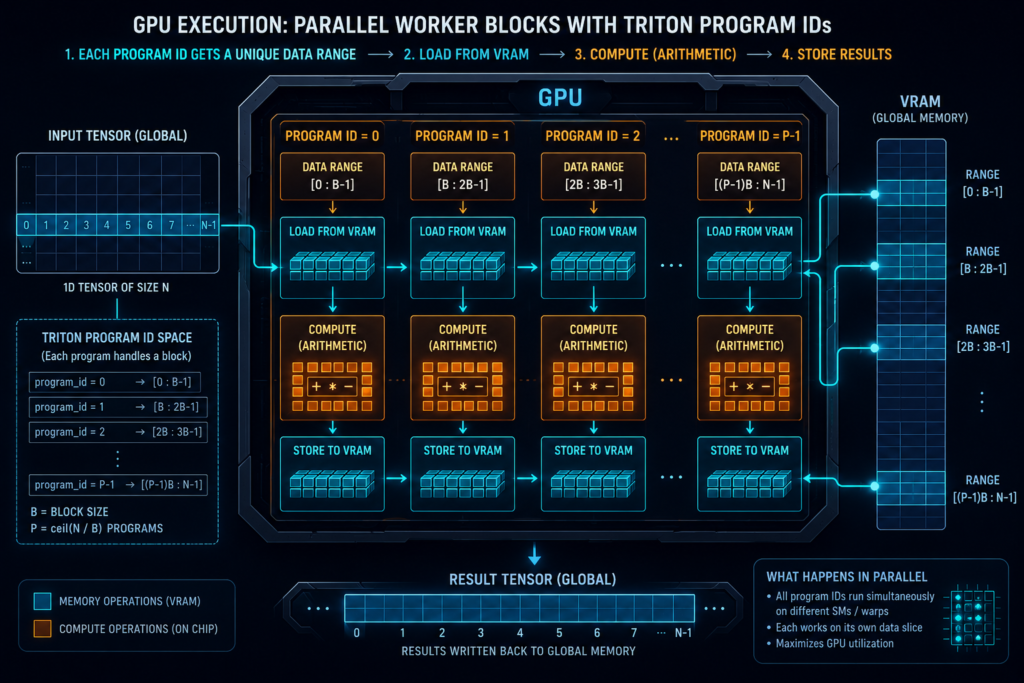
A Triton kernel doesn’t run code one element at a time like normal Python. Instead, it describes parallel GPU work across thousands of hardware threads simultaneously.
Here is a simplified Triton vector-addition kernel directly from official tutorials:
import triton
import triton.language as tl


@triton.jit
def add_kernel(
    x_ptr,
    y_ptr,
    output_ptr,
    n_elements,
    BLOCK_SIZE: tl.constexpr,
):
    pid = tl.program_id(axis=0)

    block_start = pid * BLOCK_SIZE

    offsets = block_start + tl.arange(
        0,
        BLOCK_SIZE
    )

    mask = offsets < n_elements

    x = tl.load(
        x_ptr + offsets,
        mask=mask
    )

    y = tl.load(
        y_ptr + offsets,
        mask=mask
    )

    result = x + y

    tl.store(
        output_ptr + offsets,
        result,
        mask=mask
    )
Don’t let the unfamiliar syntax intimidate you. Let’s break down what each piece does:
1. tl.program_id()
pid = tl.program_id(axis=0)
Imagine you have one million numbers to process and thousands of GPU worker teams. The pid (Program ID) acts like an ID badge telling each team their role:
You are Team 0.
You are Team 1.
You are Team 2. (and so on)
2. tl.arange()
offsets = block_start + tl.arange(
    0,
    BLOCK_SIZE
)
This calculates the exact memory positions (indices) that the current GPU worker team needs to handle.
3. tl.load()
x = tl.load(x_ptr + offsets, mask=mask)
Pulls raw data safely from the GPU’s global memory (VRAM) into fast local memory using a safety mask to avoid going out of bounds.
4. The Computation
result = x + y
Performs the actual mathematical calculation in parallel.
5. tl.store()
tl.store(output_ptr + offsets, result, mask=mask)
Writes the final calculated results back into GPU memory.
That is the fundamental anatomy of a GPU kernel: load data -> compute in parallel -> store the result.
Where Kernel Fusion Becomes Powerful ?
To understand why torch.compile() is such a game-changer, look at what happens with a simple set of math operations in normal PyTorch:
def transform(x, bias):
    x = x + bias
    x = x * 0.5
    x = torch.relu(x)
    return x
The Eager Mode Bottleneck (Without Fusion)
In normal eager execution, PyTorch runs each line independently as a separate step. That means the GPU has to perform multiple separate memory trips:
Load x & bias from VRAM → Add them → Save intermediate result back to VRAM
Load intermediate result → Multiply by 0.5 → Save next result back to VRAM
Load result → Apply ReLU → Save final output back to VRAM
Every time data bounces back and forth between the GPU’s slow global memory (VRAM) and its processing units, it creates a massive traffic jam. Even though GPUs are lightning-fast at math, they spend a lot of time waiting for data to travel back and forth.
How Kernel Fusion Fixes It :
When torch.compile() and TorchInductor analyze your code, they can fuse these compatible pointwise operations together into a single, unified workflow.
Instead of writing every intermediate step back to global VRAM, the data stays right next to the compute units in fast on-chip SRAM:
Load x & bias once
   ↓
(x + bias)
   ↓
(× 0.5)
   ↓
(ReLU)
   ↓
Store final result directly to VRAM
Why Does This Speed Things Up So Much?
The massive performance boost comes from two major wins combined:
Fewer Kernel Launches: Your CPU stops nagging the GPU with dozens of tiny individual instructions.
Less GPU Memory Traffic: Intermediate numbers don’t waste time getting written to and read from global VRAM over and over again.
As PyTorch’s official end-to-end compilation guides point out, the real secret to these speedups is cutting down Python control overhead and slashing unnecessary GPU memory reads and writes.
A Tiny Custom Fused Triton Kernel
To make the idea concrete, suppose we want:
output = torch.relu(
    (x + bias) * 0.5
)
A simplified custom Triton kernel could look like this:
import triton
import triton.language as tl


@triton.jit
def fused_kernel(
    x_ptr,
    bias_ptr,
    out_ptr,
    n_elements,
    BLOCK_SIZE: tl.constexpr,
):
    pid = tl.program_id(0)

    offsets = (
        pid * BLOCK_SIZE
        + tl.arange(0, BLOCK_SIZE)
    )

    mask = offsets < n_elements

    x = tl.load(
        x_ptr + offsets,
        mask=mask
    )

    bias = tl.load(
        bias_ptr + offsets,
        mask=mask
    )

    value = (x + bias) * 0.5

    value = tl.maximum(
        value,
        0.0
    )

    tl.store(
        out_ptr + offsets,
        value,
        mask=mask
    )
Notice what happened.
We did not create:
add kernel
multiply kernel
ReLU kernel
The mathematical chain exists inside one kernel.
This is only an educational custom example; Inductor’s generated kernels vary with hardware, shapes, data types, compiler decisions, and PyTorch version.
PyTorch torch.compile() vs Eager Simulator
Execution Controls
Live Performance Telemetry
Generated Backend Code Inspector
Python Eager Interpreter
# Eager Execution Code Stream
x = x + bias
x = x * 0.5
x = torch.relu(x)
How to Use torch.compile() Correctly ?
Let’s look at a complete, clean PyTorch neural network example to see how compilation fits into a real training loop.
The Code Example:
import torch
import torch.nn as nn

class ToyModel(nn.Module):
    def __init__(self):
        super().__init__()
        self.net = nn.Sequential(
            nn.Linear(1024, 1024),
            nn.ReLU(),
            nn.Linear(1024, 1024)
        )

    def forward(self, x):
        return self.net(x)

# 1. Initialize model on GPU
model = ToyModel().cuda()

# 2. Compile the model
# Traditionally, you might see: model = torch.compile(model)
# Current compiler guidance recommends compiling in place using the module method:
model.compile()

# 3. Set up optimizer and dummy data
optimizer = torch.optim.AdamW(model.parameters(), lr=1e-3)
x = torch.randn(32, 1024, device="cuda")

# 4. Training loop
for step in range(100):
    optimizer.zero_grad(set_to_none=True)

    output = model(x)
    loss = output.sum()

    loss.backward()
    optimizer.step()
Key Takeaways from the Code:
In-Place Compilation (
model.compile()): While the classic wrapper approach (model = torch.compile(model)) is still fully valid, the recommended method is calling.compile()directly on your top-levelnn.Module. This compiles the module in place without replacing your Python variable with an external wrapper.Efficient Gradient Clearing (
set_to_none=True): Usingset_to_none=Trueinsideoptimizer.zero_grad()is a great practice alongsidetorch.compile(), as it saves memory bandwidth by setting gradients toNoneinstead of explicitly writing zeros.
Why Are the First Calls Dramatically Slower? (The Cold Start Problem)
If you run the training loop above, you will notice that the very first few steps take significantly longer than the rest.
This happens because the first call isn’t just running math—it is performing heavy background work:
Graph capture (TorchDynamo tracing your code)
Graph optimization (AOTAutograd and graph structuring)
Code generation (TorchInductor building backend logic)
Triton compilation (Compiling custom GPU machine code)
Autotuning (Benchmarking kernel variants, if enabled)
Execution
According to PyTorch compilation documentation, cold compilation can range anywhere from a few seconds to several minutes depending on the size and complexity of your model.
Crucial Rule: Never benchmark the first compiled iteration. Always warm up your model with a few initial steps before measuring speed, otherwise, your benchmarks will look deceptively slow!
Understanding PyTorch Compile Modes Properly
When you use torch.compile(), you aren’t stuck with just one setting. PyTorch currently provides four documented compilation modes to let you balance compilation time versus raw runtime speed:
defaultreduce-overheadmax-autotunemax-autotune-no-cudagraphs
Let’s break down what the three primary modes actually do and when you should use them.
1. default Mode
model = torch.compile(
    model,
    mode="default"
)
What it does: Offers a balanced mix between compilation cost (how long it takes to start) and runtime performance.
When to use: This is where almost everyone should start. It gives you immediate speedups without making you wait forever for the code to compile.
2. reduce-overhead Mode
model = torch.compile(
    model,
    mode="reduce-overhead"
)
What it does: Uses CUDA Graphs to aggressively cut down CPU-to-GPU instruction and kernel-launch overhead.
When to use: Ideal when your GPU workload is relatively small—such as small batch sizes—where the CPU spends more time telling the GPU what to do than the GPU actually spends computing.
The Catch:
CUDA Graphs do not work on every single graph structure.
It consumes extra GPU memory because workspace memory is cached.
Rule of thumb:
reduce-overheaddoes not mean universally fastest. It means “aggressively reduce runtime launch overhead where CUDA Graph capture is possible.”
3. max-autotune Mode
model = torch.compile(
    model,
    mode="max-autotune"
)
What it does: Allows TorchInductor to spend significantly more compilation time testing and benchmarking different kernel configurations for supported operations (like trying out multiple matrix-multiplication setups to find the absolute fastest one).
The Analogy: Think of it like testing five different high-performance engine setups before a 24-hour race.
The testing cost looks ridiculous if you are only running a quick 5-second benchmark.
But if you are launching a training job that will run continuously for days, that extra startup time pays for itself.
Under the Hood: Current PyTorch documentation notes that
max-autotuneuses Triton or template-based matrix multiplications and Triton-based convolutions on GPUs, while also enabling CUDA Graphs by default.
Benchmark Eager vs. Compiled Correctly (Why Standard Timers Lie)
If you use Python’s standard time.time() to measure GPU speed, your test will give you completely wrong numbers.
Here is why: CUDA execution is asynchronous. When your Python code calls model(x), the CPU sends the instruction to the GPU and instantly moves to the next line—long before the GPU actually finishes calculating the math.
If you use time.time(), you are only measuring how fast the CPU hands off the work, not how fast the GPU does the work.
The Right Way: Using CUDA Events
To benchmark your models accurately, you must use PyTorch CUDA Events and synchronize the GPU. Here is the correct, production-grade benchmarking script:
import torch

def benchmark(
    fn,
    x,
    warmup=20,
    iterations=100,
):
    # 1. Warm up the model (Crucial for torch.compile to finish compiling!)
    for _ in range(warmup):
        fn(x)

    # Ensure all warmup operations are complete
    torch.cuda.synchronize()

    # Create precise GPU timing events
    start = torch.cuda.Event(enable_timing=True)
    end = torch.cuda.Event(enable_timing=True)

    start.record()
    for _ in range(iterations):
        fn(x)
    end.record()

    # Wait for the GPU to finish all iterations
    torch.cuda.synchronize()

    # Calculate average time per iteration in milliseconds
    total_ms = start.elapsed_time(end)
    return total_ms / iterations
Running the Comparison
Now, let’s put our benchmark function to work and compare an Eager model against a compiled model:
eager_model = ToyModel().cuda().eval()

# Compile a separate instance for testing
compiled_model = torch.compile(
    ToyModel().cuda().eval()
)

x = torch.randn(32, 1024, device="cuda")

# Run the benchmark
eager_ms = benchmark(eager_model, x)
compiled_ms = benchmark(compiled_model, x)

print(f"Eager:    {eager_ms:.3f} ms")
print(f"Compiled: {compiled_ms:.3f} ms")
print(f"Speedup:  {eager_ms / compiled_ms:.2f}x")
Why You Should Never Copy Benchmark Numbers
Never trust generic speedup claims (like “torch.compile gives a 2x boost!”) found online. Real speedup depends entirely on your specific setup:
Hardware: Which GPU are you using? (e.g., A100 vs. RTX 4090)
Model Architecture: Is it a Transformer, CNN, or simple MLP?
Batch Size & Shape: Are shapes static or dynamic?
Data Type (dtype): Are you running FP32, FP16, or BF16?
Memory Pressure & Compile Mode: Are you using
defaultorreduce-overhead?Software Versions: Which PyTorch and CUDA versions are installed?
The Golden Rule: A model heavily bottlenecked by Python overhead or VRAM memory traffic will see massive speedups with torch.compile(). However, a model that already maxes out heavy tensor compute cores may see much smaller gains. Always benchmark on your own hardware!
Graph Breaks vs. Recompilations: Know the Difference
Developers often confuse these two terms, but they mean completely different things and hurt your performance in different ways.
1. Graph Breaks (When the Compiler Has to Split Your Code)
A Graph Break happens when TorchDynamo runs into a piece of Python code or an operation it doesn’t understand (like a print statement or an unsupported library call) and is forced to stop capturing a single continuous graph.
What it looks like in code:
def example(x):
    print("Shape:", x.shape)  # ⚠️ Graph break! Print is a side effect.
    y = x * 2
    return torch.relu(y)
What happens behind the scenes:
Instead of optimizing the whole function together, the compiler breaks it into pieces:
Compiled Graph A
      ↓
Python / Unsupported Region (Slow Interpreter)
      ↓
Compiled Graph B
This destroys optimization opportunities because execution keeps jumping back and forth out of the fast compiled zone.
How to Debug Graph Breaks:
You can catch them right from your terminal:
TORCH_LOGS="graph_breaks" python train.py
Or directly inside Python using:
import torch

torch._logging.set_logs(graph_breaks=True)
You can also test a specific function using torch._dynamo.explain():
explanation = torch._dynamo.explain(example)(torch.randn(10, device="cuda"))
print(explanation)
2. Recompilations (When the Compiler Has to Rebuild the Graph)
A Recompilation is completely different. Your code might be 100% valid with zero graph breaks, but your previous compiled version becomes invalid, forcing PyTorch to waste time compiling a brand-new version from scratch.
Why it happens: When input tensor shapes or data types change unexpectedly (especially with static shapes), your compiler “Guards” stop matching.
What it looks like in code:
@torch.compile(dynamic=False)
def scale(x):
    return x * 2

# Each call with a new shape forces a painful recompilation!
scale(torch.randn(16, device="cuda"))
scale(torch.randn(32, device="cuda"))
scale(torch.randn(64, device="cuda"))
How to Debug Recompilations:
Run your training script with this log flag:
TORCH_LOGS="recompiles" python train.py
Summary Checklist :
| Performance Issue | What It Means | Quick Fix / Debug Flag |
| Graph Break | The compiler had to split your graph into multiple parts due to unsupported Python code. | TORCH_LOGS="graph_breaks" (Remove side-effects like print() inside compiled loops) |
| Recompilation | The compiler had to create a brand-new compiled version because input shapes/types changed. | TORCH_LOGS="recompiles" (Use dynamic=True if shapes vary, or pad inputs to a fixed size) |
Dynamic Shapes: Why You Should Stop Blindly Using dynamic=True
You will see this piece of advice everywhere online:
model = torch.compile(
    model,
    dynamic=True
)
“Just add dynamic=True whenever your sequence length or batch size changes.”
That advice is outdated and too simplistic.
The Default Behavior: dynamic=None
Modern PyTorch uses a smarter default:
dynamic = None
When dynamic=None, PyTorch takes a hybrid, adaptive approach:
It specializes for your initial tensor shapes first to squeeze out maximum hardware performance.
If it detects shape-driven recompilations happening repeatedly, it automatically attempts to compile more dynamic, flexible shapes behind the scenes.
Why Blanket dynamic=True is Discouraged ?
Forcing dynamic=True on everything right from the start can cause hidden issues:
Performance Regressions: Fully dynamic shapes prevent the compiler from making certain aggressive optimizations, making your execution slower.
Unnecessary Complexity: It introduces extra compilation overhead and guard checks.
The Correct Production Strategy :
Instead of blindly adding dynamic=True everywhere, follow this professional workflow:
Start clean with the default compilation:
model.compile()Investigate actual recompilations using PyTorch’s built-in logging tools if your training loop starts stuttering due to changing shapes:
TORCH_LOGS="recompiles,dynamic" python train.pyOnly enable dynamic dimensions (
dynamic=Trueor specific dynamic shapes configuration) for the exact tensors and dimensions where your workload genuinely requires it.
How to Inspect the Generated Triton Code ?
This is one of the most exciting parts of using torch.compile(). Instead of treating the compiler like a black box, you can actually look at the exact custom GPU code PyTorch generated for your model!
To see the code generated by TorchInductor, run your Python training script with this environment variable:
TORCH_LOGS="output_code" python train.py
Other Useful Logging Flags:
For individual kernels: If you want to isolate and print the generated code for each separate GPU kernel, run:
TORCH_LOGS="kernel_code" python train.pyTo combine multiple logs: You can inspect outputs, individual kernels, and fusion decisions all at once by comma-separating them:
TORCH_LOGS="output_code,kernel_code,fusion" python train.py
What Do the Terms Mean?
output_code: Prints the complete Inductor-generated code (which could include custom Triton or C++ code).kernel_code: Focuses specifically on printing the generated code broken down per kernel.
What Does the Generated Triton Code Look Like?
When you inspect the logs, you will see actual Triton JIT kernels generated automatically by PyTorch. They look something like this:
@triton.jit
def triton_(...):
    xoffset = (
        tl.program_id(0)
        * XBLOCK
    )
    xindex = (
        xoffset
        + tl.arange(0, XBLOCK)
    )

    # Loads data, applies cosine and sine, and stores result in one go
    tmp0 = tl.load(...)
    tmp1 = tl.cos(tmp0)
    tmp2 = tl.sin(tmp1)
    tl.store(...)
(This matches the exact structure shown in PyTorch’s official getting-started documentation for Inductor outputs.)
Why This Matters ?
This is the exact moment when torch.compile() stops feeling like an unexplained magic trick. You are no longer guessing whether optimization worked—you can literally read the custom GPU program that PyTorch built specifically for your code!
What About DDP (Distributed Data Parallel)?
When training models across multiple GPUs using Distributed Data Parallel (DDP), things get a bit tricky. Most tutorials give a rigid rule, but the reality requires more nuance.
Two Different Ways to Combine DDP and Compilation :
Approach 1: Compile the DDP Wrapper (Traditional)
Stable DDP documentation historically showed wrapping the model in DDP first, and then compiling it:
ddp_model = DDP(
    model,
    device_ids=[rank]
)

ddp_model = torch.compile(
    ddp_model
)
Why do this? TorchDynamo can use its built-in
DDPOptimizerand make smart graph-break decisions that are informed by DDP’s communication bucket sizes.
Approach 2: Compile the Inner Module First (Newer Guidance)
Recent compiler best practices indicate that distributed wrappers like DDP and FSDP (Fully Sharded Data Parallel) can sometimes be difficult targets for the compiler to trace directly. Instead, compiling the inner model before wrapping it in DDP is often recommended:
model.compile()

model_ddp = DDP(
    model,
    device_ids=[rank]
)
The Bottom Line on DDP & Compilation :
There is no universal rule that works for every single setup:
❌ You cannot honestly say: “Always compile before DDP.”
❌ You cannot honestly say: “Always compile after DDP.”
The Production Rule: For a real distributed workload, test both approaches on your exact PyTorch version, check your cluster telemetry, and use whichever pattern gives your specific model stable performance and clean compilation.
Production Debugging Cheat Sheet (TORCH_LOGS)
When PyTorch compilation behaves strangely or doesn’t give you the speedup you expect, guessing won’t help. Instead, use these powerful environment variables right from your terminal to inspect what the compiler is doing under the hood:
TORCH_LOGS="graph_breaks" python train.pyWhat it does: Finds where and why Python interrupted graph capture (graph breaks).
TORCH_LOGS="recompiles" python train.pyWhat it does: Flags every time changing input shapes or data types forces the compiler to re-compile your model.
TORCH_LOGS="guards" python train.pyWhat it does: Inspects the underlying assumptions (guards) the compiler made about your tensors.
TORCH_LOGS="dynamic" python train.pyWhat it does: Debugs how the compiler handles dynamic-shape decisions and variable input sizes.
TORCH_LOGS="fusion" python train.pyWhat it does: Shows you which operations were successfully combined (fused) into single kernels.
TORCH_LOGS="kernel_code" python train.pyWhat it does: Prints the actual generated Triton code for individual GPU kernels.
TORCH_LOGS="output_code" python train.pyWhat it does: Displays the complete, finalized Inductor-generated output code.
Advanced Tooling for Large Projects :
For massive codebases or complex production pipelines, PyTorch recommends using TORCH_TRACE alongside tlparse. This powerful combination generates a structured compilation report containing:
Captured execution graphs
Generated machine code
Detailed compilation metrics
Guard validation data
Frame-by-frame execution details.
The Mental Model You Should Remember
Stop thinking of torch.compile() as a magical “make my GPU go faster” switch.
Instead, view it as a complete, multi-stage compiler pipeline sitting right between your Python code and your GPU hardware, entirely reorganizing how your instructions reach the chip:
PyTorch Program
       ↓
TorchDynamo          (Captures tensor computation into a graph)
       ↓
AOTAutograd          (Supports compiled training graphs & gradients)
       ↓
TorchInductor        (Optimizes and lowers the graph into code)
       ↓
Triton Kernels       (Generates custom, hardware-specific GPU code)
       ↓
Kernel Fusion        (Combines operations: fewer launches + less VRAM traffic)
       ↓
     GPU             (Executes at maximum physical efficiency)
Keeping this exact pipeline in mind solves almost every weird behavior or mystery you will encounter while training models:
Why is the first training iteration so slow? Because of Compilation. The system is capturing graphs, running TorchInductor, compiling Triton kernels, and (if mode is set) autotuning. Never benchmark your very first step.
Why did changing your batch size or sequence length suddenly pause training? Because of a Recompilation. Your tensor shapes violated the compiler’s strict Guards, forcing it to re-compile new kernels on the fly.
Why did adding a random Python print statement or unsupported function hurt your speedup? Because of a Graph Break. Dynamo was forced to split your continuous graph into pieces, reducing optimization opportunities.
Why did three separate math expressions turn into a single GPU action? Because of Kernel Fusion. Intermediate results stayed in fast on-chip SRAM instead of bouncing back and forth to global VRAM.
Why does
mode="max-autotune"take forever to start? Because it spends extra time benchmarking multiple Triton kernel implementations to find the absolute fastest one for your specific GPU.Why does
mode="reduce-overhead"speed up small batches? Because it wraps execution in CUDA Graphs, cutting down CPU-to-GPU launch overhead.
And why should you inspect the generated Triton code at least once?
Because once you actually look at the generated code behind a simple model.compile() call, it stops feeling like an opaque black box. It transforms into what it truly is: a powerful engineering tool giving you direct, low-level control over your GPU execution.