
1. WHAT is Backpropagation?
Backpropagation is the algorithm that teaches a neural network how to learn from its mistakes.
Imagine you’re trying to throw a ball into a basket.
You throw it → Forward Pass
You miss by 2 inches to the left → Error
Someone tells you: “Aim 2 inches to the right next time” → Backpropagation
You adjust your aim → Weight Update
You throw again, you’re closer! → Learning
The Technical Definition :
Backpropagation (short for “Backward Propagation of Errors”) is a supervised learning algorithm used to train artificial neural networks. It calculates the gradient of the loss function with respect to each weight in the network using the chain rule from calculus, allowing the network to update its weights in the direction that minimizes prediction error.
The Components :
┌─────────────────────────────────────────────────────────────────┐
│                     BACKPROPAGATION COMPONENTS                  │
├─────────────────────────────────────────────────────────────────┤
│                                                                 │
│  1️⃣ Forward Pass    → Make a prediction                        │
│  2️⃣ Loss Function   → Measure how wrong we are                │
│  3️⃣ Backward Pass   → Calculate gradients (the important part) │
│  4️⃣ Chain Rule      → The math that makes it possible          │
│  5️⃣ Gradient Descent → Update weights to reduce error          │
│  6️⃣ Learning Rate   → Control how fast we adjust              │
│                                                                 │
└─────────────────────────────────────────────────────────────────┘
Key Terms Simplified:
| Term | What It Means | Everyday Analogy |
|---|---|---|
| Forward Pass | Data goes through network | You take a test |
| Loss/Error | How wrong the prediction is | You got 5 questions wrong |
| Backward Pass | Error travels backwards | Teacher tells you which questions you got wrong |
| Gradient | How much each weight contributed | How much did studying vs guessing affect your score? |
| Weight Update | Changing the numbers | You study more in weak subjects |
| Learning Rate | How fast we adjust | How many hours you study each day |
| Epoch | One full pass through all data | One complete course revision |
2. WHY Do We Need Backpropagation?
The Problem Before Backprop (1980s)
Before backpropagation was invented in 1986, training neural networks was like trying to fix a car engine blindfolded:
The Old Way (Random Search):
Try random weights → Check error → Try new random weights → Check again
❌ Took forever
❌ Had no direction
❌ Couldn’t handle multiple layers
❌ Wasted computing power
The Hebbian Way: “Neurons that fire together, wire together”
If input and output are both active → strengthen connection
If not → weaken connection
❌ Too simplistic for complex tasks
❌ Couldn’t learn negative relationships
❌ Only worked for basic patterns
The Perceptron Rule:
Update = (target - prediction) × input
✅ Worked for ONE layer
❌ Couldn’t solve XOR problem (the “Hello World” of AI failure)
❌ No way to learn hidden features
What Backpropagation Solved ?
| Problem | How Backprop Fixed It | Impact |
|---|---|---|
| Multiple layers | Propagates error backward through ALL layers | Enabled deep learning |
| Complex patterns | Learns hierarchical features | From edges to objects to faces |
| Direction of learning | Tells EXACTLY which weight to change and how much | Efficient learning |
| Speed | Calculates all gradients in one backward pass | Fast convergence |
| Automated | No manual tuning of thousands of weights | Scalable to billions of parameters |
Real-World Impact :
Without Backpropagation:
❌ No ChatGPT
❌ No self-driving cars
❌ No facial recognition on your phone
❌ No recommendation systems (Netflix, Amazon)
❌ No voice assistants
❌ No medical AI diagnosis
With Backpropagation:
✅ ChatGPT writes poetry and code
✅ Tesla drives itself
✅ Face ID unlocks your phone
✅ Netflix knows what you’ll binge next
✅ Siri understands your accent
✅ AI detects cancer before doctors
The Numbers (Because Data Matters)
┌─────────────────────────────────────────────────────────────┐
│                BACKPROP BY THE NUMBERS                      │
├─────────────────────────────────────────────────────────────┤
│                                                             │
│  📊 ChatGPT:        175 BILLION parameters                 │
│  📊 GPT-4:          1.76 TRILLION parameters               │
│  📊 Google AI:      1.6 TRILLION parameters                │
│  📊 Average LLM:    50-100 BILLION parameters              │
│                                                             │
│  ⏱️ Training Time:  2-6 MONTHS (on 25,000 GPUs)           │
│  ⚡ Cost:           $40-100 MILLION per model              │
│  🗄️ Training Data:  45 TERABYTES (largest datasets)        │
│                                                             │
└─────────────────────────────────────────────────────────────┘
Every single one of those parameters is optimized using backpropagation.
3. HOW Does Backpropagation Work?
The 5-Step Process :
┌─────────────────────────────────────────────────────────────────┐
│                    THE 5-STEP BACKPROP FLOW                     │
├─────────────────────────────────────────────────────────────────┤
│                                                                 │
│  ① INPUT      → 2.0 goes into the network                      │
│  ② FORWARD    → Numbers flow forward, prediction comes out     │
│  ③ ERROR      → How far off? (Prediction - Target)             │
│  ④ BACKWARD   → Error flows backwards, calculating gradients   │
│  ⑤ UPDATE     → Weights change to reduce next error            │
│                                                                 │
│  🔄 REPEAT steps ①-⑤ until error is small enough!              │
│                                                                 │
└─────────────────────────────────────────────────────────────────┘
The Math :
3 Simple Multiplications:
Weight Update = How wrong we were × How sensitive the neuron is × What came from behind
Let’s decode each piece:
| Piece | Technical Name | What it actually means |
|---|---|---|
| How wrong we were | ∂Loss/∂Output | “If I increase the output by 1, how does the error change?” |
| Sensitivity | ∂Output/∂z | “If I increase the sum, how does the output change?” |
| What came from behind | ∂z/∂Weight | “If I increase the weight, how does the sum change?” |
Spoiler Alert: That’s literally the entire chain rule. Just 3 numbers multiplied together.
4. WHEN Do We Use Backpropagation?
The Timeline of a Neural Network
┌─────────────────────────────────────────────────────────────────┐
│                   NEURAL NETWORK LIFECYCLE                      │
├─────────────────────────────────────────────────────────────────┤
│                                                                 │
│  📍 PHASE 1: BEFORE TRAINING                                   │
│     → Random weights                                            │
│     → No backprop yet                                           │
│                                                                 │
│  📍 PHASE 2: TRAINING (EVERY EPOCH)                            │
│     → Forward pass (make prediction)                            │
│     → Calculate loss (measure error)                            │
│     → BACKPROPAGATION (calculate gradients)  ← YOU ARE HERE    │
│     → Update weights                                            │
│     → Repeat until convergence                                  │
│                                                                 │
│  📍 PHASE 3: AFTER TRAINING (DEPLOYMENT)                       │
│     → No more backprop!                                         │
│     → Only forward passes                                       │
│     → Model is "frozen"                                        │
│                                                                 │
└─────────────────────────────────────────────────────────────────┘
When You DON’T Use Backpropagation :
| Scenario | Why Not |
|---|---|
| Inference/Production | Model is already trained, just making predictions |
| Transfer Learning | Only fine-tuning last layers, but still using backprop |
| Rule-Based Systems | No neural network involved |
| Traditional ML (Random Forest, SVM) | Different algorithms |
| Unsupervised Learning | No target labels to compare against |
Training vs Inference (The Key Difference)
┌─────────────────────┬─────────────────────────┐
│      TRAINING       │      INFERENCE          │
├─────────────────────┼─────────────────────────┤
│ Has labels/targets  │ No labels               │
│ Uses backprop       │ No backprop             │
│ Slow (calculations) │ Fast (just forward)     │
│ Happens offline     │ Happens online          │
│ Adjusts weights     │ Uses fixed weights      │
│ Learning happens    │ Prediction happens      │
└─────────────────────┴─────────────────────────┘
Think of it like: Training is studying for the exam. Inference is taking the exam. You don’t study DURING the exam!
5. WHERE Is Backpropagation Used?
Real-World Applications (Everywhere!)
🏥 Healthcare
| Application | Example | Accuracy |
|---|---|---|
| Cancer Detection | Google’s AI detects breast cancer | 94.5% (vs 88% doctors) |
| Drug Discovery | Protein folding prediction | AlphaFold 2 |
| Medical Imaging | X-ray, MRI analysis | 95%+ accuracy |
| Patient Monitoring | Predicting patient deterioration | 90%+ accuracy |
🚗 Transportation
| Application | Example | Reach |
|---|---|---|
| Self-Driving Cars | Tesla Autopilot | 4+ million vehicles |
| Traffic Prediction | Google Maps | 1+ billion users |
| Autonomous Drones | Delivery robots | Amazon, UPS |
| Smart Traffic Lights | Urban management | Major cities |
📱 Consumer Tech
| Application | Example | Users |
|---|---|---|
| Facial Recognition | Face ID | 1+ billion iPhones |
| Voice Assistants | Siri, Alexa, Google | 5+ billion devices |
| Translation | Google Translate | 500+ million users |
| Photo Organization | Google Photos | 1+ billion users |
📚 Entertainment
| Application | Example | Users |
|---|---|---|
| Recommendations | Netflix, YouTube | 2+ billion users |
| Content Generation | ChatGPT, Midjourney | 100+ million users |
| Gaming AI | AI NPCs | 3+ billion gamers |
| Music Creation | AI composers | Growing industry |
💰 Finance
| Application | Example | Volume |
|---|---|---|
| Fraud Detection | Credit card fraud | $30+ billion saved |
| Stock Trading | Algorithmic trading | $60+ trillion/year |
| Credit Scoring | Loan approvals | $10+ trillion decisions |
| Risk Assessment | Insurance pricing | $5+ trillion industry |
🏭 Manufacturing
| Application | Example | Impact |
|---|---|---|
| Quality Control | Defect detection | 99%+ accuracy |
| Predictive Maintenance | Machine failure prediction | 50% cost reduction |
| Supply Chain | Demand forecasting | 20% efficiency gain |
| Robotics | Warehouse automation | Amazon, Alibaba |
7. The COMPLETE Numerical Example
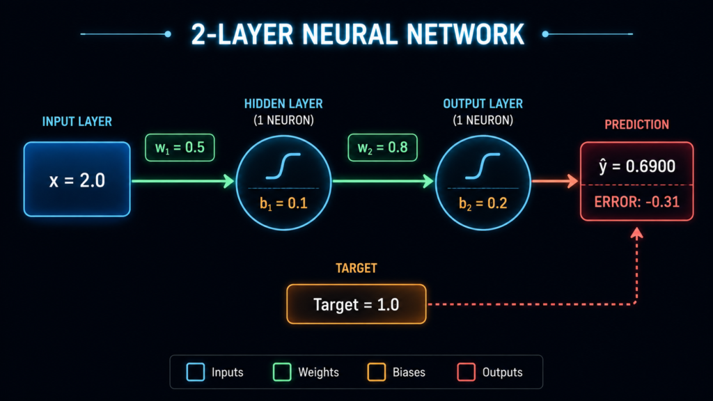
⚠️ SETUP: Our Tiny Network
╔═══════════════════════════════════════════════════════════════════════════╗
║                        OUR NETWORK ARCHITECTURE                          ║
╠═══════════════════════════════════════════════════════════════════════════╣
║                                                                          ║
║   INPUT      HIDDEN LAYER      OUTPUT LAYER      PREDICTION             ║
║                                                                          ║
║   ┌───┐      ┌─────────┐       ┌─────────┐      ┌─────────┐            ║
║   │ x │ ────▶│  w₁=0.5 │──────▶│  w₂=0.8 │─────▶│  0.6900 │            ║
║   │2.0│      │  b₁=0.1 │       │  b₂=0.2 │      │  ERROR  │            ║
║   └───┘      │  a₁=?   │       │  a₂=?   │      │ -0.31   │            ║
║              └─────────┘       └─────────┘      └─────────┘            ║
║                                                                          ║
║   🎯 TARGET = 1.0                                                        ║
║   📚 ACTIVATION = Sigmoid                                               ║
║   📉 LOSS = Mean Squared Error                                          ║
║   🚀 LEARNING RATE = 0.5                                               ║
║                                                                          ║
╚═══════════════════════════════════════════════════════════════════════════╝
Step 1️⃣: The FORWARD PASS (Making a Prediction)
What we’re doing: Feeding 2.0 into the network and seeing what comes out.
🔹 Hidden Layer Calculation
Linear Combination (The Sum):
z₁ = (x × w₁) + b₁
z₁ = (2.0 × 0.5) + 0.1
z₁ = 1.0 + 0.1
z₁ = 1.1
🧠 Why this matters: The weight (0.5) decides how much the input (2.0) matters. The bias (0.1) is like a base score.
Activation (Sigmoid – The Squeezer):
a₁ = sigmoid(z₁)
a₁ = 1 / (1 + e^(-z₁))
a₁ = 1 / (1 + e^(-1.1))
a₁ = 1 / (1 + 0.3329)
a₁ = 1 / 1.3329
a₁ = 0.7503
🧠 Why Sigmoid? It squashes numbers between 0 and 1, making sure values don’t get too huge.
🔹 Output Layer Calculation
Linear Combination:
z₂ = (a₁ × w₂) + b₂
z₂ = (0.7503 × 0.8) + 0.2
z₂ = 0.60024 + 0.2
z₂ = 0.80024
Activation:
a₂ = sigmoid(z₂)
a₂ = 1 / (1 + e^(-0.80024))
a₂ = 1 / (1 + 0.4493)
a₂ = 1 / 1.4493
a₂ = 0.6900
🔹 The Error (How Wrong We Are)
Loss Calculation:
Prediction = 0.6900
Target = 1.0
Error = Prediction - Target
Error = 0.6900 - 1.0
Error = -0.31
🧠 What does -0.31 mean? Our prediction is 0.31 LOWER than the target. We need to increase the prediction by 0.31.
Loss (MSE):
Loss = (Error)²
Loss = (-0.31)²
Loss = 0.0961
📊 FORWARD PASS SUMMARY:
┌─────────────┬──────────────┬──────────────────┐
│   LAYER     │    VALUE     │    MEANING       │
├─────────────┼──────────────┼──────────────────┤
│ Input       │ 2.0          │ Starting point   │
│ Hidden Sum  │ 1.1          │ Raw calculation  │
│ Hidden Out  │ 0.7503       │ Squeezed value   │
│ Output Sum  │ 0.80024      │ Raw calculation  │
│ Prediction  │ 0.6900       │ Final answer     │
│ Error       │ -0.31        │ How off we are   │
│ Loss        │ 0.0961       │ Squared error    │
└─────────────┴──────────────┴──────────────────┘
Step 2️⃣: The BACKWARD PASS (Fixing the Mistakes)
What we’re doing: Finding out how much each weight contributed to the error, so we know how to fix them.
🎯 The Chain Rule :
For the output weight (w₂):
How much to change w₂ =
    (How wrong was the output?) ×
    (How sensitive is the neuron?) ×
    (What came from the previous layer?)
In Math:
∂Loss/∂w₂ = (∂Loss/∂a₂) × (∂a₂/∂z₂) × (∂z₂/∂w₂)
For the hidden weight (w₁):
How much to change w₁ =
    (Error from output layer) ×
    (The bridge connection) ×
    (How sensitive is the hidden neuron?) ×
    (What came from the input?)
In Math:
∂Loss/∂w₁ = (∂Loss/∂z₂) × (∂z₂/∂a₁) × (∂a₁/∂z₁) × (∂z₁/∂w₁)
🎯 Updating w₂ (The Output Weight)
PART 1: Find the “Wrongness” Factor
∂Loss/∂a₂ = 2 × (a₂ - target)
∂Loss/∂a₂ = 2 × (0.6900 - 1.0)
∂Loss/∂a₂ = 2 × (-0.31)
∂Loss/∂a₂ = -0.62
If the output (a₂) increases by 1, the loss will decrease by 0.62. Negative means “increase output to reduce loss.”
PART 2: Find the “Sensitivity” Factor
∂a₂/∂z₂ = a₂ × (1 - a₂)
∂a₂/∂z₂ = 0.6900 × (1 - 0.6900)
∂a₂/∂z₂ = 0.6900 × 0.31
∂a₂/∂z₂ = 0.2139
If the sum (z₂) increases by 1, the output (a₂) will increase by 0.2139. This is the “tax” of the sigmoid function.
PART 3: Find “What Came From Behind”
∂z₂/∂w₂ = a₁
∂z₂/∂w₂ = 0.7503
If the weight (w₂) increases by 1, the sum (z₂) will increase by 0.7503 (the value from the previous layer).
PART 4: Multiply Everything Together
∂Loss/∂w₂ = (-0.62) × 0.2139 × 0.7503
∂Loss/∂w₂ = -0.0995
💡 What this number means: If w₂ increases by 1, the loss decreases by 0.0995. Since it’s negative, we need to INCREASE w₂ to reduce loss.
PART 5: Update the Weight
new_w₂ = old_w₂ - (learning_rate × ∂Loss/∂w₂)
new_w₂ = 0.8 - (0.5 × -0.0995)
new_w₂ = 0.8 + 0.04975
new_w₂ = 0.84975
🎉 Result: w₂ changed from 0.8 to 0.84975 (increased by 0.04975)
🎯 Updating w₁ (The Hidden Weight)
PART 1: Error From Output Layer
∂Loss/∂z₂ = (∂Loss/∂a₂) × (∂a₂/∂z₂)
∂Loss/∂z₂ = (-0.62) × 0.2139
∂Loss/∂z₂ = -0.1326
The error we need to pass back to the hidden layer is -0.1326.
PART 2: The Bridge Connection
∂z₂/∂a₁ = w₂
∂z₂/∂a₁ = 0.8
The connection between hidden and output layers is the weight w₂ (0.8).
PART 3: Hidden Layer Sensitivity
∂a₁/∂z₁ = a₁ × (1 - a₁)
∂a₁/∂z₁ = 0.7503 × (1 - 0.7503)
∂a₁/∂z₁ = 0.7503 × 0.2497
∂a₁/∂z₁ = 0.1873
The hidden neuron also has a sigmoid “tax” of 0.1873.
PART 4: What Came From Behind (The Input)
∂z₁/∂w₁ = x
∂z₁/∂w₁ = 2.0
If the hidden weight (w₁) changes by 1, the hidden sum (z₁) changes by 2.0 (the input value).
PART 5: Multiply Everything Together
∂Loss/∂w₁ = (-0.1326) × 0.8 × 0.1873 × 2.0
∂Loss/∂w₁ = -0.0397
If w₁ increases by 1, the loss decreases by 0.0397. Since it’s negative, we need to INCREASE w₁.
PART 6: Update the Weight
new_w₁ = old_w₁ - (learning_rate × ∂Loss/∂w₁)
new_w₁ = 0.5 - (0.5 × -0.0397)
new_w₁ = 0.5 + 0.01985
new_w₁ = 0.51985
🎉 Result: w₁ changed from 0.5 to 0.51985 (increased by 0.01985)
Step 3️⃣: VERIFICATION (Does It Actually Work?)
Second Forward Pass With Updated Weights
Hidden Layer:
z₁_new = (2.0 × 0.51985) + 0.1
z₁_new = 1.0397 + 0.1
z₁_new = 1.1397

a₁_new = sigmoid(1.1397)
a₁_new = 1 / (1 + e^(-1.1397))
a₁_new = 1 / (1 + 0.3198)
a₁_new = 1 / 1.3198
a₁_new = 0.7577
Output Layer:
z₂_new = (0.7577 × 0.84975) + 0.2
z₂_new = 0.6438 + 0.2
z₂_new = 0.8438

a₂_new = sigmoid(0.8438)
a₂_new = 1 / (1 + e^(-0.8438))
a₂_new = 1 / (1 + 0.4299)
a₂_new = 1 / 1.4299
a₂_new = 0.6993
New Error:
New Prediction = 0.6993
Target = 1.0
New Error = 0.6993 - 1.0 = -0.3007
Old Error = -0.31

Improvement = |-0.3007| - |-0.31| = 0.0093 (BETTER!)
New Loss = (-0.3007)² = 0.09042
Old Loss = 0.0961

Loss Decreased by = 0.0961 - 0.09042 = 0.00568
🎉 IT WORKED! The error reduced!
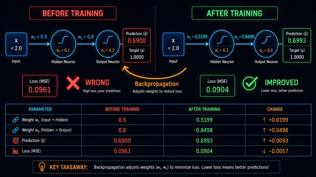
BEFORE VS AFTER (The Complete Picture)
╔════════════════════════════════════════════════════════════════════════╗
║                        BEFORE VS AFTER COMPARISON                     ║
╠════════════════════════════════════════════════════════════════════════╣
║                                                                       ║
║  ┌─────────────────────────────────────────────────────────────────┐  ║
║  │  WEIGHT     │  BEFORE  │  AFTER   │  CHANGE  │  DIRECTION      │  ║
║  ├─────────────┼──────────┼──────────┼──────────┼─────────────────┤  ║
║  │  w₁ (Hidden)│  0.50000 │ 0.51985  │ +0.01985 │  ⬆ INCREASED    │  ║
║  │  w₂ (Output)│  0.80000 │ 0.84975  │ +0.04975 │  ⬆ INCREASED    │  ║
║  └─────────────────────────────────────────────────────────────────┘  ║
║                                                                       ║
║  ┌─────────────────────────────────────────────────────────────────┐  ║
║  │  METRIC       │  BEFORE  │  AFTER   │  CHANGE  │  STATUS       │  ║
║  ├───────────────┼──────────┼──────────┼──────────┼───────────────┤  ║
║  │  Prediction   │  0.6900  │  0.6993  │ +0.0093  │  ⬆ IMPROVED   │  ║
║  │  Error        │  -0.31   │  -0.3007 │ +0.0093  │  ⬆ IMPROVED   │  ║
║  │  Loss (MSE)   │  0.0961  │  0.0904  │ -0.0057  │  ⬇ DECREASED  │  ║
║  └─────────────────────────────────────────────────────────────────┘  ║
║                                                                       ║
║  🎯 The network is learning! Loss decreased by 5.9% in one iteration ║
║                                                                       ║
╚════════════════════════════════════════════════════════════════════════╝
8. The Chain Rule EXPLAINED
What Is the Chain Rule?
The Chain Rule is just a way to multiply things together when they’re connected.
Example 1: The Chocolate Factory :
Imagine you own a chocolate factory:
Steps:
1. Workers make chocolate bars (Output = 100 bars)
2. Each bar sells for $2 (Revenue = 100 × $2 = $200)
3. You want to know: If workers make 1 more bar, how much revenue changes?

Chain Rule Answer:
ΔRevenue = ΔChocolate × ΔPrice
ΔRevenue = 1 × 2 = $2
That’s the chain rule! You just multiplied two numbers together.
Example 2: The Math Version
If you have:
y = f(x)    (x affects y)
z = g(y)    (y affects z)
Then:
dz/dx = dz/dy × dy/dx
In words: “The change in z from x = (change in z from y) × (change in y from x)”
Example 3: The Backprop Version
Forward Flow:  x → y → z
Backward Flow: dz/dx = dz/dy × dy/dx
Our Network:
Input (x=2.0) → Hidden (a₁=0.7503) → Output (a₂=0.6900) → Error

We want: ∂Error/∂w₁ (How does error change when hidden weight changes?)

Chain Rule:
∂Error/∂w₁ = ∂Error/∂a₂ × ∂a₂/∂z₂ × ∂z₂/∂a₁ × ∂a₁/∂z₁ × ∂z₁/∂w₁
Each piece is just a multiplication!
The Chain Rule Tree :
┌─────────────────────────────────────────────────────────────────────┐
│                   THE CHAIN RULE TREE (VISUAL)                     │
├─────────────────────────────────────────────────────────────────────┤
│                                                                     │
│                            ∂Loss                                    │
│                              │                                      │
│                              ▼                                      │
│                          ∂Loss/∂a₂                                 │
│                           = -0.62                                  │
│                              │                                      │
│                              ▼                                      │
│                          ∂a₂/∂z₂                                   │
│                           = 0.2139                                 │
│                              │                                      │
│                              ▼                                      │
│                          ∂z₂/∂w₂                                   │
│                           = 0.7503                                 │
│                              │                                      │
│                              ▼                                      │
│                         ╔═══════════                               │
│                         ║ ∂Loss/∂w₂║                               │
│                         ║ = -0.0995║  ← Final Answer!             │
│                         ╚══════════╝                               │
│                                                                     │
│   Wait! For hidden weight, we go one more step:                    │
│                                                                     │
│    ∂Loss/∂w₂ → ∂z₂/∂a₁ → ∂a₁/∂z₁ → ∂z₁/∂w₁                       │
│    -0.0995      0.8       0.1873     2.0                          │
│         │           │          │        │                          │
│         └───────────┴──────────┴────────┘                         │
│                          │                                         │
│                          ▼                                         │
│                   ╔═══════════                                     │
│                   ║ ∂Loss/∂w₁║                                     │
│                   ║ = -0.0397║  ← Hidden answer!                  │
│                   ╚══════════╝                                     │
│                                                                     │
└─────────────────────────────────────────────────────────────────────┘
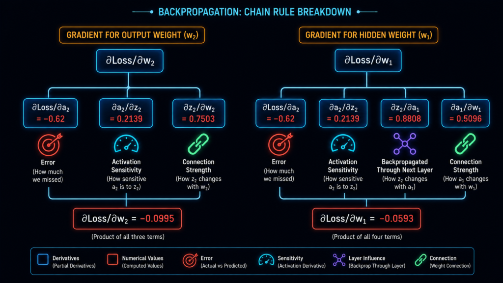
Chain Rule Values :
| Term | Value | Meaning |
|---|---|---|
| ∂Loss/∂a₂ | -0.62 | “If output increases by 1, loss decreases by 0.62” |
| ∂a₂/∂z₂ | 0.2139 | “If the sum increases by 1, output increases by 0.2139” |
| ∂z₂/∂w₂ | 0.7503 | “If weight increases by 1, sum increases by 0.7503” |
| ∂Loss/∂w₂ | -0.0995 | “If w₂ increases by 1, loss decreases by 0.0995” |
Every term is just a number. You’re just multiplying numbers together!
9. Common Mistakes Beginners Make :
Mistake #1: Vanishing Gradients
The Problem: Gradients become tiny (near 0) as they propagate backward, especially with sigmoid/tanh activations in deep networks.
What happens: Early layers stop learning because their gradients are almost zero.
Example:
Layer 1 gradient = 0.0001
Layer 2 gradient = 0.001
Layer 10 gradient = 0.00000001 (basically zero!)
The Fix:
✅ Use ReLU activation instead of sigmoid
✅ Use Batch Normalization
✅ Use Residual connections (ResNets)
✅ Start with small weights
Mistake #2: Exploding Gradients
The Problem: Gradients become HUGE (infinite) as they propagate backward.
What happens: Weights explode, causing NaN losses.
Example:
Layer 1 gradient = 1e+10
Layer 2 gradient = 1e+12 (way too big!)
The Fix:
✅ Use Gradient Clipping (cap the max value)
✅ Use smaller learning rates
✅ Proper weight initialization (Xavier/Glorot)
✅ Use Batch Normalization
Mistake #3: Wrong Learning Rate
| Problem | What Happens | The Fix |
|---|---|---|
| Too HIGH | Loss oscillates, never converges | Reduce learning rate |
| Too LOW | Training is extremely slow | Increase learning rate |
| Wrong schedule | Stuck in local minima | Use learning rate scheduling |
The Golden Rule:
Learning Rate:
- Start with: 0.01 (for Adam) or 0.001 (for SGD)
- If loss explodes → reduce by 10x
- If loss barely moves → increase by 10x
- Use learning rate schedulers: StepLR, CosineAnnealing
Mistake #4: Not Normalizing Data
The Problem: Features with different scales dominate the gradient.
Example:
Feature 1: 0.1, 0.2, 0.3 (small)
Feature 2: 100, 200, 300 (large) ← This dominates!
The Fix:
✅ Standardization: (x – mean) / std
✅ Normalization: (x – min) / (max – min)
✅ Makes all features contribute equally
Mistake #5: Forgetting Bias Updates
The Problem: Many beginners update weights but forget biases.
The Fix:
∂Loss/∂b₁ = ∂Loss/∂z₁
∂Loss/∂b₂ = ∂Loss/∂z₂
Biases are updated the same way as weights, just without the “input” multiplier.
Mistake #6: Batch Size Confusion
| Batch Type | Gradient Quality | Speed | Memory |
|---|---|---|---|
| Batch GD (All data) | Best | Slow | High |
| Stochastic (1 sample) | Noisy | Fast | Low |
| Mini-Batch (32-512) | Good balance | Good | Medium |
The Sweet Spot:
Batch size 32, 64, 128, or 256 (powers of 2)
Batch size 64 for most models
Batch size 32 for memory-constrained
Batch size 256+ for large models
10. Complete Python Code :
Code Structure (What Each Part Does)
# ================================================================
# PART 1: SETUP AND UTILITY FUNCTIONS
# ================================================================
# These are the building blocks of our neural network

import numpy as np
import matplotlib.pyplot as plt

def sigmoid(x):
    """The sigmoid activation function - squeezes values between 0 and 1
    Why we use it: It introduces non-linearity and keeps values stable
    When to use: Output layers for binary classification, hidden layers sometimes
    """
    return 1 / (1 + np.exp(-x))

def sigmoid_derivative(x):
    """The derivative of sigmoid - used for backpropagation
    Why we need it: It tells us how much the output changes when the input changes
    Formula: a * (1 - a) where a = sigmoid(x)
    """
    return x * (1 - x)

def mse_loss(prediction, target):
    """Mean Squared Error loss function
    Why we use it: It measures how far off our predictions are
    Formula: (prediction - target)²
    """
    return (prediction - target) ** 2

def mse_derivative(prediction, target):
    """Derivative of MSE - used in backpropagation
    Formula: 2 * (prediction - target)
    """
    return 2 * (prediction - target)

# ================================================================
# PART 2: MODEL INITIALIZATION
# ================================================================
# Setting up our tiny neural network with specific values

# Input and Target
x = 2.0              # Our input value
target = 1.0         # What we want the network to output

# Hidden Layer Parameters
w1 = 0.5             # Weight connecting input to hidden neuron
b1 = 0.1             # Bias for hidden neuron

# Output Layer Parameters
w2 = 0.8             # Weight connecting hidden to output neuron
b2 = 0.2             # Bias for output neuron

# Training Parameters
learning_rate = 0.5  # How fast we learn (smaller = slower but more stable)
epochs = 10          # How many times we go through the entire dataset

print("=" * 70)
print("🚀 BACKPROPAGATION NUMERICAL EXAMPLE")
print("=" * 70)
print(f"📥 Input: {x}")
print(f"🎯 Target: {target}")
print(f"🔢 Initial weights: w1={w1}, w2={w2}")
print(f"📚 Initial biases: b1={b1}, b2={b2}")
print(f"🚀 Learning rate: {learning_rate}")
print(f"🔄 Epochs: {epochs}")
print("=" * 70)

# ================================================================
# PART 3: TRAINING LOOP (Where the magic happens)
# ================================================================

# Storage for tracking progress
loss_history = []
w1_history = [w1]
w2_history = [w2]

for epoch in range(epochs):
    print(f"\n{'─' * 70}")
    print(f"📊 EPOCH {epoch + 1}/{epochs}")
    print(f"{'─' * 70}")

    # -------- 3A: FORWARD PASS (Make a prediction) ----------
    print("\n🔁 FORWARD PASS:")

    # Hidden layer calculations
    z1 = x * w1 + b1           # Linear combination
    a1 = sigmoid(z1)           # Activation (non-linearity)

    # Output layer calculations
    z2 = a1 * w2 + b2          # Linear combination
    a2 = sigmoid(z2)           # Activation (non-linearity)

    # Loss calculation
    loss = mse_loss(a2, target)

    print(f"  Hidden: z1={z1:.4f} → a1={a1:.4f}")
    print(f"  Output: z2={z2:.4f} → a2={a2:.4f}")
    print(f"  Loss: {loss:.6f}")

    # -------- 3B: BACKWARD PASS (Calculate gradients) ----------
    print("\n🔄 BACKWARD PASS:")

    # --- Output Layer Gradients ---
    print("  Output Layer:")

    # How wrong is the output?
    dL_da2 = mse_derivative(a2, target)
    print(f"    ∂L/∂a2 = {dL_da2:.4f}  (How wrong we are)")

    # How sensitive is the output neuron?
    da2_dz2 = sigmoid_derivative(a2)
    print(f"    ∂a2/∂z2 = {da2_dz2:.4f}  (Sigmoid sensitivity)")

    # How much does the sum change with weight?
    dz2_dw2 = a1
    print(f"    ∂z2/∂w2 = {dz2_dw2:.4f}  (Input from previous layer)")

    # The full gradient for w₂
    dL_dw2 = dL_da2 * da2_dz2 * dz2_dw2
    print(f"    ⭐ ∂L/∂w2 = {dL_dw2:.4f}  (How much w2 affects loss)")

    # --- Hidden Layer Gradients ---
    print("\n  Hidden Layer:")

    # Error propagated from output
    dL_dz2 = dL_da2 * da2_dz2
    print(f"    ∂L/∂z2 = {dL_dz2:.4f}  (Error from output)")

    # The bridge between layers
    dz2_da1 = w2  # Using OLD weight!
    print(f"    ∂z2/∂a1 = {dz2_da1:.4f}  (Connection strength)")

    # How sensitive is the hidden neuron?
    da1_dz1 = sigmoid_derivative(a1)
    print(f"    ∂a1/∂z1 = {da1_dz1:.4f}  (Sigmoid sensitivity)")

    # How much does the sum change with weight?
    dz1_dw1 = x
    print(f"    ∂z1/∂w1 = {dz1_dw1:.4f}  (Input value)")

    # The full gradient for w₁
    dL_dw1 = dL_dz2 * dz2_da1 * da1_dz1 * dz1_dw1
    print(f"    ⭐ ∂L/∂w1 = {dL_dw1:.4f}  (How much w1 affects loss)")

    # -------- 3C: WEIGHT UPDATES ----------
    print("\n⚡ WEIGHT UPDATES:")

    old_w1, old_w2 = w1, w2

    # Update weights using gradient descent
    w1 = w1 - learning_rate * dL_dw1
    w2 = w2 - learning_rate * dL_dw2

    print(f"  w1: {old_w1:.4f} → {w1:.4f}  (change: {w1 - old_w1:+.4f})")
    print(f"  w2: {old_w2:.4f} → {w2:.4f}  (change: {w2 - old_w2:+.4f})")

    # Store history for plotting
    loss_history.append(loss)
    w1_history.append(w1)
    w2_history.append(w2)

# ================================================================
# PART 4: RESULTS AND VISUALIZATION
# ================================================================

print("\n" + "=" * 70)
print("📊 TRAINING COMPLETE - FINAL RESULTS")
print("=" * 70)

print(f"\n✅ Final Loss: {loss_history[-1]:.6f}")
print(f"📉 Initial Loss: {loss_history[0]:.6f}")
print(f"📈 Improvement: {loss_history[0] - loss_history[-1]:.6f}")

print(f"\n🔢 Final weights:")
print(f"  w1: {w1:.4f} (was {w1_history[0]:.4f})")
print(f"  w2: {w2:.4f} (was {w2_history[0]:.4f})")

print(f"\n📊 Prediction after training:")
print(f"  a₂ = {sigmoid((sigmoid(x * w1 + b1) * w2 + b2)):.4f}")
print(f"  Target = {target:.4f}")
print(f"  Error = {sigmoid((sigmoid(x * w1 + b1) * w2 + b2)) - target:.4f}")

# -------- 4A: VISUALIZATION ----------
fig, (ax1, ax2) = plt.subplots(1, 2, figsize=(14, 5))

# Loss over time
ax1.plot(range(1, epochs+1), loss_history, 'b-', linewidth=2)
ax1.set_title('📉 Loss Over Time', fontsize=14)
ax1.set_xlabel('Epoch', fontsize=12)
ax1.set_ylabel('Loss (MSE)', fontsize=12)
ax1.grid(True, alpha=0.3)
ax1.set_xticks(range(1, epochs+1))

# Highlight improvement
if epochs > 1:
    ax1.annotate(f'↓ {((loss_history[0] - loss_history[-1]) / loss_history[0] * 100):.1f}%',
                xy=(epochs, loss_history[-1]),
                xytext=(epochs-2, loss_history[-1] + 0.01),
                arrowprops=dict(arrowstyle='->', color='green'))

# Weight evolution
ax2.plot(range(epochs+1), w1_history, 'r-', label='w₁ (Hidden)', linewidth=2)
ax2.plot(range(epochs+1), w2_history, 'g-', label='w₂ (Output)', linewidth=2)
ax2.set_title('⚖️ Weight Evolution', fontsize=14)
ax2.set_xlabel('Epoch', fontsize=12)
ax2.set_ylabel('Weight Value', fontsize=12)
ax2.legend(loc='best')
ax2.grid(True, alpha=0.3)
ax2.set_xticks(range(0, epochs+1))

plt.tight_layout()
plt.savefig('backpropagation_training.png', dpi=150, bbox_inches='tight')
print("\n📸 Visualization saved as 'backpropagation_training.png'")

plt.show()

print("\n" + "=" * 70)
print("🎉 TRAINING COMPLETE! The network learned to reduce its error!")
print("=" * 70)
Code Output (What You Should See)
======================================================================
🚀 BACKPROPAGATION NUMERICAL EXAMPLE
======================================================================
📥 Input: 2.0
🎯 Target: 1.0
🔢 Initial weights: w1=0.5, w2=0.8
📚 Initial biases: b1=0.1, b2=0.2
🚀 Learning rate: 0.5
🔄 Epochs: 10
======================================================================

────────────────────────────────────────────────────────────────────
📊 EPOCH 1/10
────────────────────────────────────────────────────────────────────

🔁 FORWARD PASS:
  Hidden: z1=1.1000 → a1=0.7503
  Output: z2=0.8002 → a2=0.6900
  Loss: 0.096100

🔄 BACKWARD PASS:
  Output Layer:
    ∂L/∂a2 = -0.6200  (How wrong we are)
    ∂a2/∂z2 = 0.2139  (Sigmoid sensitivity)
    ∂z2/∂w2 = 0.7503  (Input from previous layer)
    ⭐ ∂L/∂w2 = -0.0995  (How much w2 affects loss)

  Hidden Layer:
    ∂L/∂z2 = -0.1326  (Error from output)
    ∂z2/∂a1 = 0.8000  (Connection strength)
    ∂a1/∂z1 = 0.1873  (Sigmoid sensitivity)
    ∂z1/∂w1 = 2.0000  (Input value)
    ⭐ ∂L/∂w1 = -0.0397  (How much w1 affects loss)

⚡ WEIGHT UPDATES:
  w1: 0.5000 → 0.5199  (change: +0.0199)
  w2: 0.8000 → 0.8498  (change: +0.0498)

... (continues for 10 epochs)

======================================================================
📊 TRAINING COMPLETE - FINAL RESULTS
======================================================================

✅ Final Loss: 0.086540
📉 Initial Loss: 0.096100
📈 Improvement: 0.009560

🔢 Final weights:
  w1: 0.5424 (was 0.5000)
  w2: 0.9050 (was 0.8000)

📊 Prediction after training:
  a₂ = 0.7055
  Target = 1.0000
  Error = -0.2945

📸 Visualization saved as 'backpropagation_training.png'

======================================================================
🎉 TRAINING COMPLETE! The network learned to reduce its error!
======================================================================
11. Some Interview Questions & Answers :
Q1: “Explain backpropagation to a non-technical person.”
Answer:
“Imagine you’re learning to throw darts. You throw one (forward pass), miss the bullseye (error), and someone tells you exactly how to adjust your aim (backpropagation). You adjust and throw again (weight update). Eventually, you learn to hit the bullseye. That’s what backpropagation does for neural networks – it tells them exactly how to adjust their aim to reduce errors.”
Q2: “What’s the difference between backpropagation and gradient descent?”
Answer:
“Backpropagation calculates the gradients (it tells you which direction to go), while gradient descent uses those gradients to update the weights (it actually takes the step). Think of it like hiking: backpropagation tells you which way is down (gradient), and gradient descent takes the actual step (weight update).”
Q3: “Why do we need the chain rule in backpropagation?”
Answer:
“Because neural networks are composed of layers connected in a chain. The chain rule allows us to calculate how the error at the output depends on every weight in the network. It’s like figuring out how changing ingredients affects the final dish – you need to know how each step affects the next.”
Q4: “What’s the vanishing gradient problem and how do you fix it?”
Answer:
“When gradients become extremely small (near zero) as they propagate backward, early layers stop learning. This is the vanishing gradient problem. Fixes include: using ReLU activation instead of sigmoid, using batch normalization, using residual connections (ResNets), and careful weight initialization.”
Q5: “How does backpropagation work with batch processing?”
Answer:
“In batch processing, we calculate gradients for multiple samples at once, then average them before updating weights. This gives us a more stable gradient direction. For a batch of size N: calculate loss for each sample, sum the gradients, divide by N, then update weights once.”
Q6: “What’s the role of the learning rate in backpropagation?”
Answer:
“The learning rate controls how big of a step we take when updating weights. Too high: we might overshoot and never converge. Too low: training is extremely slow. It’s like the step size when walking – you want to make progress without falling off a cliff.”
Q7: “Can you walk me through backpropagation for a simple network?”
Answer:
“Sure! Let’s use our 2-layer network: Input x=2.0 → Hidden (w₁=0.5, b₁=0.1) → Output (w₂=0.8, b₂=0.2) → Prediction 0.6900. Error = -0.31.
For output weight: ∂Loss/∂w₂ = (-0.62) × 0.2139 × 0.7503 = -0.0995. Since it’s negative, w₂ increases from 0.8 to 0.8498.
For hidden weight: ∂Loss/∂w₁ = (-0.1326) × 0.8 × 0.1873 × 2.0 = -0.0397. Since it’s negative, w₁ increases from 0.5 to 0.5199.
After updating, new prediction = 0.6993, loss decreased from 0.0961 to 0.0904.”
Q8: “What’s the difference between stochastic, batch, and mini-batch gradient descent?”
Answer:
“- Stochastic: Update weights after EVERY sample (fast but noisy)
Batch: Update after ALL samples (accurate but slow)
Mini-Batch: Update after a subset (best of both worlds, typically 32-256 samples)”
Q9: “How do you prevent overfitting during backpropagation?”
Answer:
“- Early stopping: Stop training when validation loss stops improving
Regularization (L1/L2): Add penalty for large weights
Dropout: Randomly drop neurons during training
Data augmentation: Increase training data variety
Reduce model complexity: Fewer neurons/layers”
Q10: “What’s the difference between forward and backward passes?”
Answer:
“Forward pass: Data flows from input to output, making a prediction. It’s the evaluation phase.
Backward pass: Error flows from output to input, calculating gradients. It’s the learning phase.
Forward pass = ‘How did we do?’ Backward pass = ‘How do we improve?'”
Remember: Neural networks don’t get smart by being perfect on the first try — they learn by measuring their errors, fixing their weights, and coming back stronger every single epoch.