Why Your RAG Pipeline Finds the Right Topic (And the Wrong Answer)

You ask your AI search:

“Which restaurants in Delhi do NOT have outdoor seating?”

Your vector database searches through millions of files and confidently returns:

• Best rooftop cafes in Delhi

• Top outdoor dining spots in Connaught Place

• Restaurants with beautiful garden patios

Everything looks semantically relevant. And everything is completely wrong.

You check your vector DB—it’s fine. You check your embeddings—they are state-of-the-art. You check your LLM—it’s not hallucinating.

So what the hell is going on?

You just hit the most expensive, most misunderstood trap in modern AI engineering: Semantic similarity is not the same thing as relevance.

Your vector search found the right neighborhood, but it walked you straight into the wrong house. Let’s fix your retrieval architecture.

Act 1: The Mechanics (Why “Smart” Search is Actually Dumb)

Before we build, we need to understand the two engines powering your retrieval.

The Bi-Encoder: The Speed Demon.

A bi-encoder (or dual-encoder) processes your query and your documents independently.

Query → [Encoder] → Vector A
Document → [Encoder] → Vector B
Similarity = Cosine(Vector A, Vector B)

The Superpower: Pre-computation.

If you have 10 million documents, you don’t run the model 10 million times per query. You run it once, cache the vectors in a database (like Qdrant, Pinecone, or Milvus), and just do fast math at query time. This is why semantic search scales.

The Kryptonite: The “NOT” Problem.

A vector is a compressed summary. When you squash a whole document into 768 or 1024 dimensions, fine-grained details get blurred. (Note: Modern instruction-tuned models like BGE or E5 handle negation much better than older ones, but they still struggle with complex, multi-constraint logic).

If the query is “restaurants WITHOUT outdoor seating”, the bi-encoder sees the heavy semantic weight of “restaurants” and “outdoor seating” and says, “Close enough!”

The Cross-Encoder: The Precision Sniper

The cross-encoder throws the independence out the window. It concatenates the query and the document and processes them together in a single transformer pass.

[CLS] Query [SEP] Document [SEP] → [Encoder] → Relevance Score (0.94)

The Superpower: Deep Interaction.

Because the query and document are in the same attention mechanism, the model can literally look at the word “NOT” in the query and attend to the word “outdoor” in the document. It doesn’t just ask, “Are these similar?” It asks, “Does this document actually satisfy this specific constraint?”

The Kryptonite: The Quadratic Cost.

You can’t pre-compute cross-encoder scores. The score depends on the pair.
If you have 1 query and 10 million documents, a cross-encoder requires 10 million forward passes. It will melt your GPU and your latency budget.

The Verdict:
They aren’t competitors. They’re a relay team.
Bi-encoders find the neighborhood. Cross-encoders pick the exact house.

Act 2: The Architecture (Building the Retrieve-then-Rerank Pipeline)

If you just use a bi-encoder, you get speed but lose precision.
If you just use a cross-encoder, you get precision but lose scale.

Production RAG combines them. But we need to add one more piece to the puzzle: Hybrid Search.

Why Dense Retrieval Isn’t Enough ?

Semantic search is great for vibes. It’s terrible for exact identifiers.

If a user searches for “Error E_CONN_RESET_1047”, a bi-encoder might return documents about “network timeouts” because they are semantically close. But the user needs the exact string. This is why modern pipelines use Hybrid Search:

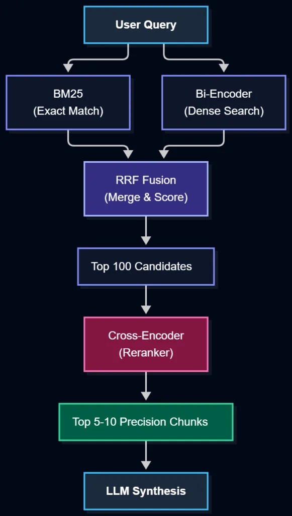
BM25 (Sparse): Catches exact keywords and identifiers.
Dense (Bi-Encoder): Catches semantic concepts.
Reciprocal Rank Fusion (RRF): Merges the two lists into a single candidate pool.

The Pipeline :
Here is the actual architecture you should be building:

The Code :

Here’s how this looks in Python. Notice we aren’t just doing naive numpy arrays; we are thinking about batching and real-world flows.

from sentence_transformers import SentenceTransformer, CrossEncoder, util
import torch

# 1. Initialize Models
bi_encoder = SentenceTransformer("BAAI/bge-large-en-v1.5")
reranker = CrossEncoder("BAAI/bge-reranker-v2-m3")

# Dummy corpus for demonstration
corpus = [
"Best rooftop cafes in Delhi with outdoor seating.",
"Top outdoor dining spots in Connaught Place.",
"Restaurants with beautiful garden patios.",
"Cozy indoor-only bistros in Delhi with no outdoor seating.",
"Delhi restaurants that do NOT have outdoor seating.",
"Guide to outdoor seating in Delhi."
]

query = "Which Delhi restaurants do NOT have outdoor seating?"

# STAGE 1: BI-ENCODER RETRIEVAL
corpus_embeddings = bi_encoder.encode(corpus, convert_to_tensor=True)
query_embedding = bi_encoder.encode(query, convert_to_tensor=True)

hits = util.semantic_search(query_embedding, corpus_embeddings, top_k=3)
candidate_indices = [hit['corpus_id'] for hit in hits[0]]
candidate_docs = [corpus[i] for i in candidate_indices]

print("--- Stage 1: Bi-Encoder Top 3 (Flawed) ---")
for i, doc in enumerate(candidate_docs):
print(f"{i+1}. {doc}")

# STAGE 2: CROSS-ENCODER RERANKING
pairs = [(query, doc) for doc in candidate_docs]
scores = reranker.predict(pairs, batch_size=32, show_progress_bar=False)

# STAGE 3: RE-SORT AND TAKE THE BEST
ranked_results = sorted(
zip(scores, candidate_docs),
key=lambda x: x[0],
reverse=True
)

print("\n--- Stage 2: Cross-Encoder Reranked (Fixed) ---")
for score, doc in ranked_results:
print(f"[{score:.4f}] {doc}")

The Golden Rule of Reranking:

Act 3: The Evolution (Agentic RAG, ColBERT, and the Latency Reality)

Once you build a basic search pipeline, you will hit production bottlenecks. Let’s break down how to handle speed, scale, and advanced models without breaking your app.

1. The Latency Reality Check: Why More Top-K Can Break Your App

Reranking is powerful, but it is not free. Let’s look at a realistic millisecond (ms) breakdown for a single search query:

• Vector Search (Bi-Encoder): ~20 ms

• Cross-Encoder Rerank (Top 50 docs): ~100 ms

• LLM Answer Generation: ~800 ms

• Total Latency: ~920 ms (Fast and smooth!)

The Trap: What happens when your RAG misses a document, and you panic, turning your Top-K from 50 up to 500 to “catch everything”? Your cross-encoder now has to process 10x more text pairs. Your reranking time jumps from 100ms to 1,000ms+, pushing your total user wait time past 2 seconds.

• The Takeaway: Tuning Top-K is a strict engineering trade-off between recall accuracy and speed, not a magic button you turn up infinitely.

2. Enter ColBERT: The “Middle Child” of Retrieval

When standard dense vectors are too blurry and cross-encoders are too slow, engineers turn to Late Interaction models, most famously ColBERT.

How do the three architectures compare?

• Bi-Encoder: Creates 1 vector per document. Super fast because it pre-computes everything, but blurs out fine details.

• Cross-Encoder: Processes query and document together. Extremely precise, but too slow for millions of raw files.

• ColBERT (Late Interaction): Keeps a separate vector for every single token in your document.

At query time, ColBERT uses a smart scoring trick called MaxSim. Instead of crushing a whole document into one vector, it compares every single word (token) in your query against every word in your document, finding the maximum matches.

• Why it matters: It gives you the deep, laser-focused precision of a cross-encoder while keeping the pre-computation speed of a bi-encoder. If your production app demands instant speed and deep word-level matching, ColBERT is definitely worth exploring.

3. Agentic RAG: When Search Becomes a Loop

1. Searches for current policy.
2. Searches for historical policy.
3. Reranks the results to ensure the dates match the constraints.
4. If the reranker scores are too low, the agent realizes: “My evidence is weak. Let me rewrite the query and search again.”